Webster R., Oliver M.A., Geostatistics for Environmental Scientists

Подождите немного. Документ загружается.

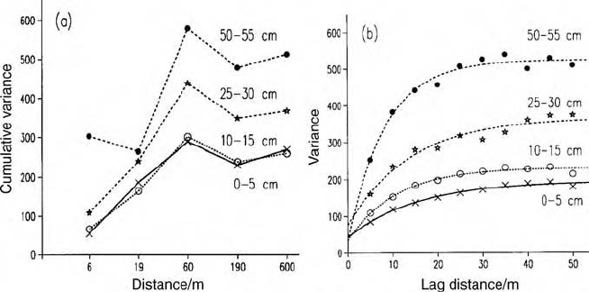
against separating distance on a logarithmic scale to give ﬁrst approximations

to the variograms. The graph shows that at least 80% of the variation at the

four depths for sand content occurs within 60 m; this was the case for all of the

other properties. Stages 1 and 2, i.e. distances of 190–600 m and 60–190 m,

respectively, account for less than 20% of the variation. The estimated

components of variance for stage 2 were generally negative. This suggests

that either there is some repetition in soil character at that distance, or that the

components estimate zero because there is no contribution to the variance at

this stage. The conﬁdence limits of the components are wide, and so we cannot

be sure how to interpret these negative values. Even at stage 5 there is still a

considerable con tribution to the total variance. This represents the unresolved

variation within 6 m plus errors of measurement.

Let us now look at the estimates of the variance components by REML.

Table 6.9 lists the results, ﬁrst without any constraint and then with the

estimates constrained to be non-negative. The unconstrained estimates are

somewhat different from those from ANOVA, but they show the same general

pattern. Constraining the estimates to a minimum of 0 caused little change in

the positive compon ents in the lowest stage, but appreciable changes in all

stages above those that were negative in the unconstrained analysis.

As described above, the experimental variogram depends on the spat ial scale

over which we measure it. If a large extent is covered with wide sampling

intervals then all of the variance might appear as nugget. Alternatively, if small

intervals are chosen to resolve the short-range variance then the sampling

required to estimate the contributions to the larger distances would be too

costly. A nested survey identiﬁes the scale at which most of the variation occurs

Figure 6.16 Variograms of soil properties in the Wyre Forest: (a) obtained by

accumulation of the components of variance estimated by REML, with the lag distance

on a logarithmic scale; (b) estimated from subsequent transect sampling at 5 m intervals.

Theory of Nested Sampling and Analysis 137

at the level of our investigation. The reconnaissance variograms for the soil

properties of the Wyre Forest showed that most of the spatial variation occurred

over dist ances less than 60 m.

From this information we could design a survey to estimate the variogram

more precisely by linear sampling. We did so using ten transects each 100 m

long and one of 500 m with a sampling interval of 5 m. The conventional

variograms that resulted, Figure 6.16(b), showed correlation extending to little

more than about 40 m.

We could have used the results of the nested survey to design an overall

survey with a m aximum sampling interval equal to half the correlation range

identiﬁed. This would have been 30 m. In the event, having estimated the

variograms more precisely along transects and established an effective range of

40 m, we sam pled at a 20-m interval from which to interpolate for mapping.

You can read a full account in Oliver and Webster (1987).

6.2.5 Summary

Nested survey and analysis can reveal the spatial scale(s) of variation in a

region with modest sampling effort. The data can be analysed by straightfor-

ward analysis of variance for balanced designs or, preferably, by residual

maximum likelihood for unbalanced ones. We recommend it as a ﬁrst step in

the description of variation in a hitherto little known region. Armed with the

results, one can plan a second stage of survey to estimate the vari ogram

precisely over the range that matters. The results from nested survey could be

used to plan a regional survey if one particu lar component proved dominant.

Table 6.9 Components of variance of sand content of the soil at four depths in the

survey of the Wyre Forest, estimated by REML without constraints and constrained to be

non-negative.

Component of variance Constrained variance

Depth/cm Depth/cm

Stage 0–5 10–15 25–30 50–55 0–5 10–15 25–30 50–55

1 (600 m) 38.12 21.07 18.68 33.75 19.70 0.44 0 0

2 (190 m) 58.03 63.17 90.02 100.19 0 0 0 0

3 (60 m) 102.50 137.58 198.51 314.81 63.58 96.06 125.26 235.89

4 (19 m) 131.50 97.65 131.95 38.89 131.43 97.65 131.03 0

5 (6 m) 54.97 66.54 108.56 303.26 54.88 66.27 109.87 276.06

138 Reliability of the Experimental Variogram and Nested Sampling

Spectral Analysis

In some places the land varies laterally in a regular fashion. The most obvious

regular patterns are man-made. They include the characteristic ridge and

furrow of the English clay lands, and orch ards and plantations in which fruit

trees and other crops are arranged in lines with constant intervals between

them. The dynamic properties of the soil are likely to vary in tune with them

and so also have a regularity. Forest is established on peaty soil by planting

young trees on the upt urned sod after deep ploughing in lines. Less obvious are

the long-lasting patterns of former ploughing on crop yield, revealed by

McBratney and Webster (1981), and the effects of earlier drainage schemes

on the present-day soil described by Burrough et al. (1985). In all these the

regularity is deliberate.

Natural features may also seem regular. Examples are the frost polygons of

the Arctic region and their fossil relics in the Northern tem perate zone (e.g.

Hodge and Seale, 1966), the patterns of termite mounds in Africa, especially

evident on some of the East African plains (e.g. Scott et al., 1971) and in the

miombo woodland of Zambia and Congo and the gilgai of Australia (e.g.

Hallsworth et al., 1955; Webster, 1977).

The experimental variograms of such patterns ﬂuctuate with evident peri-

odicity, as Webster (1977) discovered. Other periodic patterns can arise from

cultivation and land management (McBratney and Webster, 1981; Burrough

et al., 1985). Chapter 5 mentioned basic periodic functions that might be used

to describe the ﬂuctuation, but we deferred illustration until now so that we can

deal with it and spectral analysis together.

7.1 LINEAR SEQUENCES

More often than not we encounter periodicity in linear, i.e. one-dimensional,

sequences of data comprising records made at regular intervals in either time or

Geostatistics for Environmental Scientists/2nd Edition R. Webster and M.A. Oliver

# 2007 John Wiley & Sons, Ltd

space (see, for example, Oliver et al., 1997). Spatial examples include:

 photographic and radiometric survey by aircraft;

 bathymetric and son ar survey from ships;

 electric logs of boreholes for oil exploration ;

 pollen counts through peat;

 isotope measurements through polar ice;

 transect surveys of soil.

In some instances each line is one of several or many in R

or R

. In others the

lines are isolated repr esentatives of two-dimensional scenes. Variables, such as

temperature, may also be recorded at regular intervals in time, and in that

instance there is only one dimension. We can analyse the data by all of the

standard geostatistical methods described above. However, if there is periodicity

then it is often proﬁtable to express the variation in relation to frequency rather

than space or time, and this takes us into the realm of spectral analysis.

7.2 GILGAI TRANSECT

To illustrate an analysis of periodic variation we use the data from a survey by

Webster (1977) of salinit y on the Bland Plain of eastern Australia. This

virtually ﬂat plain is part of the Murray–Darling Basin. Its soil is dominantly

clay, but with a more sandy surface horizon of variable thickness, alkaline and

locally saline. One of its most remarkable features is its patterns of gilgai. The

gilgais are small, almost circular depressions from a few centimetres to as much

as 50 cm deep in the plain and several metres across. The soil in their bottoms is

usually clay and wetter than that elsewhere.

A paddock at Caragabal, NSW, was sampled at regular 4-m intervals along a

transect almost 1.5 km long. At each of 365 samplin g points a core of soil,

75 mm in diameter, was taken to 1 m, and segments of it were analysed in the

laboratory. For present purposes we shall concern ourselves with just one

variable, the electrical conduc tivity at 30–40 cm. Table 7.1 sum marizes the

data, which were strongly skewed and therefore transformed to logarithms for

further analysis. Figure 7.1 shows the logarithm of conductivity plotted against

position as the ﬁne line. The bold line is a smooth ing spline ﬁtted to the data to

ﬁlter out the short-range variation and reveal a ﬂuctuation of longer range that

appears regular.

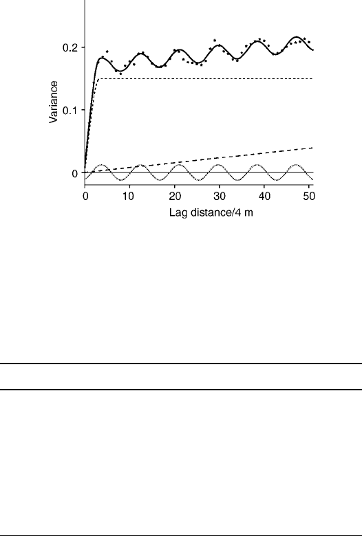
The experimental variogram of the data is shown in Figure 7.2 as the plotted

points, to which we have ﬁtted a model with a periodic component. The full

model is given by

gðhÞ¼c

þ wh þ cfsphðaÞg þ c

cos

2ph



þ c

sin

2ph



: ð7:1Þ

140 Spectral Analysis

It comprises a small nugget, c

, a linear component, wh, a spherical function

with a short range, cfsphðaÞg, and a sine wave, c

cosð2ph=vÞþc

sinð2ph=vÞ.

The values of these parameters are given in Table 7.2. The sph erical component

contributes most to the variance, with a sill of approximately 0.15

log

(mS cm

1

). It represents repetitive variation of a kind that is not periodic.

For present purposes the periodic component, though representing less of the

variance with an amplitude of only 0.012, is of most interest. Its wavelength is

8.67 sampling units or 35 m. This is approximately equal to the average

distance between the centres of the gilgai on the transect. It has a phase shift of

0:43 rad (about 25



). The linear component has only a very gentle gradient;

it is of little practical consequence, and we may regard the underlying variation

log conductivity

1.5

1.0

0.5

–0.5

–1.0

–1.5

0 100 200 300

Postition/4 m

Figure 7.1 Trace of common logarithm of electrical conductivity at Caragabal (ﬁne

line) with a smoothing spline (bold) added as an aid to see the suspected periodicity.

Table 7.1 Summary statistics of electrical conductivity in the soil at

30–40 cm at Caragabal.

Electrical conductivity

mS cm

1

log

(mS cm

1

)

Minimum 0.06 1:214

Maximum 5.10 0.707

Mean 0.958 0:2298

Median 0.54 0:2668

Variance 0.95948 0.19205

Standard deviation 0.975 0.438

Skewness 1.642 0.101

Gilgai Transect 141

as second-order stationary. The nugget variance is also very small. In passing,

we note that the periodic component does not damp, and so the model is valid

in one dimension only.

7.3 POWER SPECTRA

Let us now consider how to examin e this variation in the frequency domain.

We start by assuming that the underlying variable, ZðxÞ, is random, spatially

correlated, and second-order stationary. Since we are dealing with only one

Figure 7.2 Variogram of log electrical conductivity. The points are the sample values,

the heavy line is the ﬁtted model comprising the four components shown with the lighter

lines. The parameter values are listed in Table 7.2.

Table 7.2 Parameter values of model ﬁtted to variogram of log

electrical conductivity in the soil at 30–40 cm at Caragabal. Distances

are in sampling intervals of 4 m, and angles are in radians.

Component Parameter Value

Nugget constant, c

0.01760

Linear gradient, w 0.000772

Spherical sill, c 0.1498

range, a 3.323

Periodic amplitude, W, 0.01230

wavelength, v 8.667

phase, f 0:435

0:01116

0.005181

142 Spectral Analysis

dimension for the tim e being, we can replace x by x ¼jxj and h by h ¼jhj. Its

covariance function, in the notation of Chapter 4, is

CðhÞ¼E½fZðxÞmgfZðx þ hÞmg ¼ E½ZðxÞZðx þ hÞm

; ð7:2Þ

where m is the mea n of the process.

The covariance function in the spatial domain has an equivalent in the

frequency domain where the variance, instead of being a function of distance

(or time), is distributed as a function of frequency, f . This function, denoted by

Rðf Þ, is the spectrum,orpower spectrum. It is the Fourier transform of the

covariance function deﬁned for the interval from positions X=2toX=2, i.e.

X=2  ZðxÞX=2:

Rðf Þ¼ lim

X!1

2X

f1 ðjhj=2XÞgexpðjfhÞCðhÞdh; ð7:3Þ

where j is

ﬃﬃﬃﬃﬃﬃﬃ

1

. Provided CðhÞ approaches 0 as h approaches 1, the limiting

value of Rðf Þ is given by

Rðf Þ¼

1

expðjfhÞCðhÞd h: ð7:4Þ

The covariance function is symmetric; it is an ‘even’ function of h, i.e.

CðhÞ¼CðhÞ; see Chapter 4. As a consequence, the complex term in the

integral in equation (7.4) can be replaced by a simple cosine, and Rðf Þ reduces

Rðf Þ¼

1

cosðfhÞCðhÞd h: ð7:5Þ

Just as the spectrum, Rðf Þ, is the Fourier transform of the covariance

function, the latter, CðhÞ, is the Fourier transform of Rðf Þ:

CðhÞ¼

1

cosðfhÞRðf Þdf : ð7:6Þ

In other words, the relation is invertible.

We can equally well transform the autocorrelation function, r ðhÞ¼CðhÞ=Cð0Þ,

to obtain the normalized spectrum:

rðf Þ¼

1

cosðfhÞrðhÞdh: ð7:7Þ

This relation too is invertible.

Power Spectra 143

7.3.1 Estimating the spectrum

Equations (7.4) and (7.5) above deﬁne the spectrum of a real continuous

second-order stationary random process in R

. We want now to estimate the

spectrum. As in the example of the gilgai transect, we hav e data,

zðx

Þ; zðx

Þ; ...; zðx

Þ, at regular intervals on a line. The value N is the length

of the series, and replaces X to accord with geostatistical convention. From the

data we compute

CðhÞ¼

N  h

Nh

i¼1

fzðiÞ



zgfzði þ hÞ



zg; ð7:8Þ

where the zðiÞ and z ði þ hÞ are observed values, and



z is the average of the data

in the sequence, and by incrementing h one step at a tim e we obtain the

experimental covariance function. Thus the lag, h, is in units of the sampling

interval.

This set of covariances can be transformed to the corresponding experimental

spectrum by

Rðf Þ¼

Cð0Þþ2

L1

k¼1

CðkÞwðkÞcosðpfkÞ

()

ð7:9Þ

for frequency, f, in the range 0 to

cycle. In this equation L is the maximum lag

from which the transform is computed and k is the lag.

The quantity L can be regarded as the width of a ‘window’ through which the

covariance is viewed for transformation, and it is for us to choose it. We could set

it to the maximum possible from the data. We know from experience that as the

lag increases so the experimental covariances become increasingly unreliable,

and in Chapter 4 we suggested that the covariance be computed to a lag of no

more than about one-ﬁfth of the total length of a series. If we incorporate the

uncertainty in estimating CðhÞ at long lags in equation (7.9) then we shall obtain

detail in the computed spectrum that is untrustworthy. In fact, the longer is L,

the more detailed is the spectrum and the less reliable is that detail. On the other

hand, if we choose too small a value of L then we shall lose detail that might be

signiﬁcant. The window is effectively a smoothing function, and the narrower it

is in the spatial domain the more precise are the estimates at the expense of

greater bias and loss of detail. So the choice of L is always a compromise.

Some of the ﬂuctuation in the spectrum that arises from choosing a large L

can be diminished by changing the ‘shape’ of the window. The window in

equation (7.9) is rectangular (see Figure 7.3). If jkjL then CðkÞ carries weight

1=L, otherwise its weight is 0:

ðkÞ¼

1=L for 0 jkjL;

0 for jkj > L:



ð7:10Þ

144 Spectral Analysis

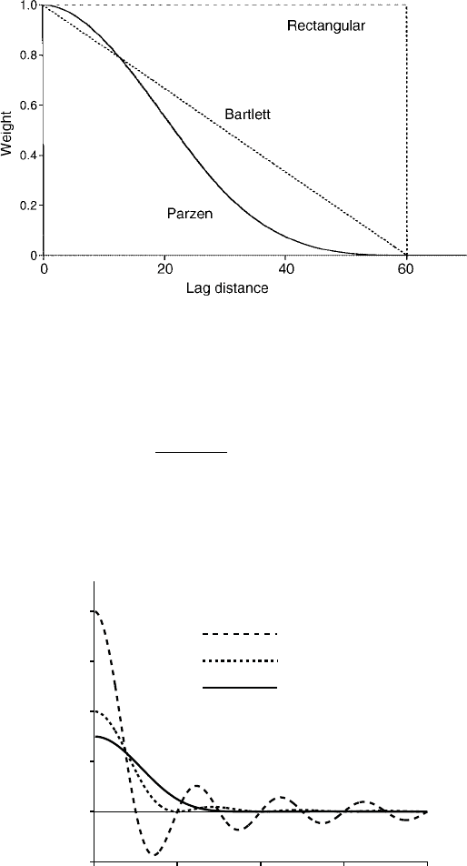
It is symmetric about the ordinate, and so we show only the positive half. Its

Fourier transform is given by

ðf Þ¼2L

sinð2pfLÞ

2pfL



for 1  f 1: ð7:11Þ

The transform of the rectangular lag window ﬂuctuates as the frequency increases

with a period of 1=L; the power takes a long while to damp. This is shown in

Figure 7.4 in which there are several peaks of decreasing height. In the jargon of

Figure 7.3 Rectangular, Bartlett and Parzen lag windows, with a basal width of 60

sampling intervals.

Rectangular

Bartlett

Parzen

012

Frequency

Spectral estimator

2.0

1.5

1.0

0.5

–0.5

Figure 7.4 Rectangular, Bartlett and Parzen spectral windows. These are the Fourier

transforms of the lag windows shown in Figure 7.3.

Power Spectra 145

spectral analysis, the rectangular window is ‘leaky’, and it is generally regarded as

unsatisfactory. The top corners of the rectangles tend to contribute most of the

leakage. This leakage can be diminished substantially by cutting the corners.

Much research has been devoted to ﬁnding an optimal shape, ‘window

carpentry’ as Jenkins and Watts (1968) called it. The simplest solution is due

to Bartlett (1966) and is known as the Bartlett window. It is deﬁned in the

spatial domain as follows:

ðkÞ¼

1 ðjkj=LÞ for 0 jkjL;

0 for jkj > L:



ð7:12Þ

The Bartlett lag window may be envisaged as an isosceles triangle with its peak

at its centre and its height decaying linearly to its lower corners where jkj of

equation (7.9) equals L. It is shown in Figure 7.3 for 0  k  L. Like the spectral

window, the lag window is symmetrical about the ordinate, and so again only

the positive half is shown. It is incorporated in the transformation equation as

Rðf Þ¼

Cð0Þþ2

L1

k¼1

CðkÞw

ðkÞcosðpfkÞ

()

: ð7:13Þ

The Fourier transform of the Bartlett lag window is

ðf Þ¼L

sinð2pfLÞ

2pfL



for 1  f 1; ð7:14Þ

and this is shown in Figure 7.4. It ﬂuctuates rather less than the rectangular

window, but nevertheless is not entirely satisfactory because of its leakage. Two

other popular windows are those deﬁned by J. W. Tukey (see Blackman and

Tukey, 1958) and Parzen (1961), and these too are referred to by the ir authors’

names. A shortcoming of Tukey’s window is that it can return negative

estimates of the spectral density, which must be positive. Parzen’s window is

more reliable. Its deﬁnition is

ðkÞ¼

1  6



þ6

jkj



for 0 jkjL=2;

21

jkj



for L=2 < jkjL;

0 for jkj > L;:

ð7:15Þ

and its Fourier transform is

ðf Þ¼

sinðpfL=2Þ

pfL=2



for 1  f 1: ð7:16Þ

146 Spectral Analysis