Webster R., Oliver M.A., Geostatistics for Environmental Scientists
Подождите немного. Документ загружается.


common logarithms to stabilize their variances, and an isotropic experimental
variogram was computed. It appears as the plotted points in Figure 5.15. Any
smooth curve through the points will have an intercept, so we include a nugget
variance in the model. By fitting single spherical and exponential functions,
with weights proportional to the numbers of pairs, we obtain the cur ves of best
fit shown in Figure 5.15(a) and (b), respectively. Clearly both fit poorly near the
ordinate. The values of the parameters, the residual sum of squares and
^
A are
listed in Table 5.2, from which it is evident that the exponential function is the
better. If we add another spherical or exponential component we obtain
the more detailed curves in Figure 5.15(c) and (d), respectively. Now the
double spherical is evidently the best, with the smallest mean squared residual.
It also has the smallest
^
A, and so in this instance we choose this more elaborate
model.
This solution is valid for weighted least-squares fitting provided the weights
remain constant, as when they are simply set in proportion to the numbers of
paired comparisons.
Webster and McBratney (1989) discuss the AIC in some detail, show its
equivalence to an F test for nes ted models, and suggest other possible criteria.
Another method for judging the goodness of a model is cross-validation. This
involves comparing kriged estimat es and their variances, and we defer it until
we have described kriging.
Table 5.2 Models fitted to the variogram of log
10
Cu in the Borders Region, estimates
of their parameters, the mean squared residual (MSR), and the variable part of the
Akaike information criterion ð
^
AÞ. The symbols are as defined in the text.
Distance
Sills parameters/km
Model c
0
c
1
c
2
a
1
a
2
r
1
r
2
MSR
^
A
Spherical 0.05027 0.01805 18.0 0.06822 128:3
Exponential 0.04549 0.02403 6.65 0.06046 134:3
Double
spherical 0.02767 0.02585 0.01505 2.7 20.5 0.02994 165:4
Double
exponential 0.00567 0.04566 0.01975 0.59 9.99 0.03616 155:7
Fitting Models 107

6
Reliability of the
Experimental Variogram
and Nested Sampling
We mentioned in Chapters 4 and 5 the importance of estimating the variogram
accurately and of modelling it correctly. This chapter deals with factors that
affect the reliability of the experimental variogram, in particular the statistical
distribution of the data, the effect of sample size on the confidence we can have
in the variogram, and the imp ortance of a suitable separating interval between
sampling points. In addition to our aim to estimate the regional variogram
reliably, we show how to use limited resources wisely to dete rmine suitable and
affordable sampling intervals.
6.1 RELIABILITY OF THE EXPERIMENTAL VARIOGRAM
Apart from the matter of anisotropy, equation (4.40) provides asymptotically
unbiased estimates of gðhÞ for Z in the region of interest, R. However, the
experimental variogram obtained will fluctuate more or less, and so will its
reliability. We now examine factors that affect these.
6.1.1 Statistical distribution
We made the point in Chapter 2 that sample variances of strongly asymmetric
or skewed (typically g
1
1org
1
1) variables are unstable. The estimates
obtained with the usual method-of-moments formula for the variogram,
equation (4.40), are variances and so are sensitive to departures from a normal
distribution. If the distribution of the variable is skewed then the confidence
limits on the variogram are wider than they would be otherwise and as a result
Geostatistics for Environmental Scientists/2nd Edition R. Webster and M.A. Oliver
# 2007 John Wiley & Sons, Ltd
the semivariances are less reliable. Skewness can result from a long upper or
lower tail in the underlying process or from the presence of a secondary process
that contaminates the primary process—values from the latter may appe ar as
outliers. Kerry and Oliver (2007a, 2007b) have studied the effects of asym-
metry in the underlying process and outliers on the variogram using simulated
fields. We summarize their results below.
Methods of estimating variograms reliably from skewed data have been
sought, and it is clear that the cause of asymmetry affects what one should
do. If the skewness coefficient exceeds the bounds given above then the
histogram or box-plot should be exam ined to reveal the deta il of the asymmetry.
In addition to these usual graphical methods, you can identify exceptional
contributions to the semivariances by drawing an h-scattergram for a given
lag, h. As described in Chapter 4, an h-scattergra m is a graph in which the zðxÞ
are plotted against the zðx þ hÞ with which they are compared in computing
^
gðhÞ. In general, the plotted points appear as more or less inflated clusters, as in
the usual kind of scatter graph.
Underlying asymmetry or skewness
Where asymmetry arises from a long tail, especially a long upper tail, in the
distribution ‘standard best practice’ has been to transform the data, as described
in Chapter 2. The variogram is then computed on the transformed data.
Transformation is not essential, however; the variogram computed from the
original data and predictions using it are unbiased, though they are not
necessarily the most precise. Perhaps more surprising is that the characteristic
form of the variogram may be changed little by transformation. So, you should
examine the experimental variograms of both raw and transformed data before
deciding which to work with.
Kerry and Oliver (2007a) explored the effects of varying skewness and sample
size, and of different transformations on random fields created by simulated
annealing (see Chapter 12 for a description of the method). They simulated
values on a square 5-m grid of 1600 points from a spherical function (equation
(5.24)), with a range, a, of 75 m, a total sill variance, c
0
þ c, of 1, and
nugget:sill ratios of 0, 0.25, 0.5, 0.75 and 1. They simulated similar fields of
400 points and 100 points with grid intervals of 10 m and 20 m, respectively.
Values in the fields were raised to a power a to create a long upper tail in the
distribution. Five values of a were used to give skewness coefficients, g
1
, of 0.5,
1.0, 1.5, 2.0 and 5.0. Here we illustrate what can happen with their results for
a ¼ 75 m, c
0
¼ 0 and c ¼ 1.
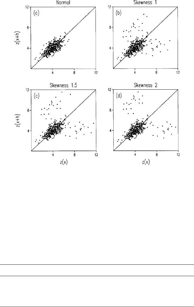
Figure 6.1 shows the h-scattergrams at lag 10 m (lag 1) from four fields
simulated on a 10 m grid. Each field has a unique coefficient of skewness,
g
1
¼ 0; 1:0; 1:5 and 2.0, caused by underlying asymmetry. The scatter of points
for the normal distribution is clustered fairly tightly along the diagonal line in
Figure 6.1(a). As the coefficient of skewness increases, the scatter becomes more
110 Reliability of the Experimental Variogram and Nested Sampling

dispersed for the larger values in the tail of the distribution reflecting the
positive skew, Figure 6.1(b)–(d). Table 6.1 lists the values of
^
rðhÞ and
^
gðhÞ for
the comparisons from these fields. The correlation coefficients decrease some-
what with inc reasing skewness, and the semivariances increase correspond-
ingly. The effects of underlying asymmetry at the first lag interval are evident,
but they are not remarkable.
Figure 6.1 The h-scattergrams for simulated fields of 400 points with underlying
asymmetry resulting in coefficients of skewness of (a) 0, (b) 1.0, (c) 1.5, (d) 2.0.
Table 6.1 Autocorrelation coefficients and semivariances for lag distance 10 m (lag 1)
computed from data simulated on a 10-m grid with four degrees of underlying skewness.
Skewness coefficient Autocorrelation coefficient Semivariance
0 0.7188 0.2700
1.0 0.6990 0.2863
1.5 0.6860 0.2984
2.0 0.6739 0.3093
Reliability of the Experimental Variogram 111
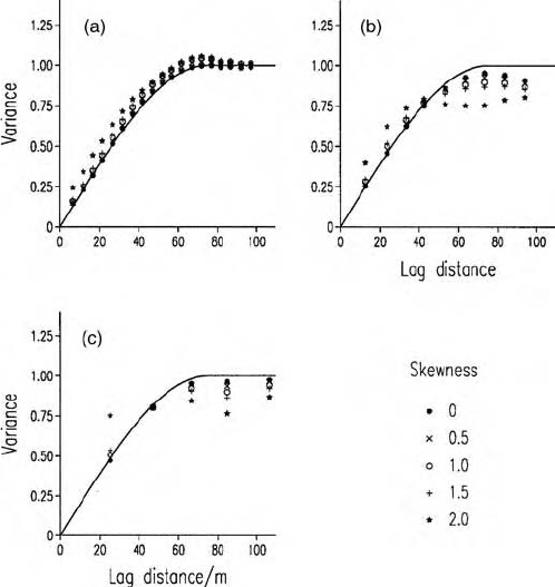
Omnidirectional variograms c omputed from the simulated fields by the
method of moments are displayed in Figure 6.2. Figure 6.2(a) shows that as
asymmetry increases the change in shape of the variogram is small for the field
on a 5 m grid. This was true even for g
1
¼ 5:0 (not shown). For the sample size
of 400 (10 m grid) the change in the shapes of the variograms is not
large, Fig ure 6. 2( b), e xc ept f or g
1
¼ 2:0. For the smaller coefficients the
semivariances are close to the generating function for the first five lags, but
beyond these they depart progessively from the sill of the generating
model. For the sample size of 100 (20-m grid), shown in Figure 6.2(c), the
semivariances at the first two lags are similar to the generating model for
g
1
¼ 0:5, 1.0, 1.5 and 2.0, but beyond this they depart progressively more
from t he sill varian ce of 1. T he variog ram compu te d from data with g
1
¼ 5:0
appeared as pure nugget. Evidently the effect of asymmetry decreases as the
sample size increases; it is greatest for the sample of 100 points and least for
that with 1600.
Figure 6.2 Experimental variograms (shown by point symbols) computed from
simulated fields of various sizes: (a) 1600 points (5-m grid), (b) 400 points (10-m
grid), (c) 100 points (20-m grid), with skewness caused by underlying asymmetry. The
solid lines represent the spherical generating function.
112 Reliability of the Experimental Variogram and Nested Sampling
Kerry and Oliver (2007a) found that transformation conferred little advan-
tage for large sets of data. Therefore, you should assess the desirability of any
transformation by com paring the variograms of raw and transformed data
visually before deciding whether to transform. In general, if there are no
marked differences between the shapes of the experimental variograms then
work on the raw data. This advice applies in particular if your aim is prediction,
for then the predicted values will be on the original scale of measurement,
which is what most practitioners want, and no back-transformation is needed
(see Chapter 8).
Outliers
The variogram is sensitive to outliers and to extreme values in general.
Histograms and box-plots, as described in Chapter 2, will usually reveal outliers
in the marginal distributions if they are present. All outliers must be regarded
with suspicion and investigated. Erroneous values should be corrected or
excised, and values that remain suspect are best removed, too. If by removing
one or a very few values you can reduce the skewness then it is reasonable to do
so to avoid the need for transformation or the use of robust variogram
estimators. For contaminated sites it is the exceptionally large values that are
often of interest. In this situation the variogram can be computed without the
outliers to ensure its stability, and then the values can be reinstated for
estimation and other analyses. Some practitioners remove the 98th or even
the 95th percentiles. This is too prescriptive in our view, and only values that
are obvious outliers should be removed.
It will be evident from equation (4.40) that each observed zðxÞ can contribute
to several estimates of gðhÞ. So one exceptionally large or small zðxÞ will tend to
swell
^
gðhÞ wherever it is compared with other values. The result is to inflate the
average. The effect is not uniform, how ever. If an extreme is near the edge of
the regi on it will contribute to fewer comparisons than if it is near the centre.
The end point on a regular transect, for example, contributes to the average just
once for each lag, whereas points near the mid dle contribute many times. If
data are unevenly scattered then the relative contributions of extreme values
are even less predictable. The result is that the experimental variogram is not
inflated equally over its range, and this can add to its erratic appearance.
Kerry and Oliver (2007b) examined the effect of outliers on the variogram for
skewness coefficients 0, 0.5, 1.0, 1.5, 2.0 and 3.0, and for randomly located
and grouped outliers. They created normally distributed data by simulated
annealing as above for the same sizes of field. These primary fields were then
contaminated by randomly located and spatially aggregated out liers from a
secondary process.
Figure 6.3 shows four h-scattergrams at lag 10 m (lag 1), from four fields
simulated on a 10-m grid with random ly located outliers to give coefficients of
skewness g
1
¼ 0, 1.0, 1.5 and 2.0. The scatter of points becomes more
Reliability of the Experimental Variogram 113
pronounced as the skewness increases from a normal distribution. For a
coefficient of skewness of 1.0, Figure 6.3(b), there is already a wide scatter of
points around a central core that represents the primary Gaussian population.
For g
1
¼ 2:0 there are now two distinct groups of points, separated from the
main group, that reflect the contaminating population. Table 6.2 supports these
Figure 6.3 The h-scattergrams for a simulated primary Gaussian field of 400 points
contaminated by outliers to give coefficients of skewness (a) 0, (b) 1.0, (c) 1.5, (d) 2.0.
Table 6.2. Autocorrelation coefficients and semivariances for lag distance 10 m (lag 1)
computed from data simulated on a 10-m grid with skewness caused by outliers.
Skewness coefficient Autocorrelation coefficient Semivariance
0 0.7188 0.270
1.0 0.3938 1.013
1.5 0.3122 1.429
2.0 0.2476 1.942
114 Reliability of the Experimental Variogram and Nested Sampling
graphical observations; the corr elation coefficients diminish markedly as skew-
ness caused by outliers increases, and also the sem ivariances increase drama-
tically.
The results in Figures 6.1 and 6.3 show how different the effects are from
different causes of asymmetry. They add strength to the statement above that
different solutions are likely to be required.
Kerry and Oliver (2007b) computed variograms as before by Matheron’s
method of momen ts and also by three robust variogram estimators proposed by
Cressie and Hawkins (1980), Dowd (1984) and Genton (1998). The estimator
of Cressie and Hawkins (1980),
^
g
CH
ðhÞ, essentially damps the effect of outliers
from the secondary process. It is based on the fourth root of the squared
differences and is given by
2
^
g
CH
ðhÞ¼
1
mðhÞ
P
mðhÞ
i¼1
jzðx
i
Þzðx
i
þ hÞj
1
2
4
0:457 þ
0:494
mðhÞ
þ
0:045
m
2
ðhÞ
: ð6:1Þ
The denominator in equation (6.1) is a correction based on the assumption that
the underlying process to be estimated has normally distributed differences over
all lags.
Dowd’s (1984) estimator,
^
g
D
ðhÞ, and Genton’s (1998 ),
^
g
G
ðhÞ, estimate the
variogram for a dominant intrins ic process in the presence of outliers. Dowd’s
estimator is given by
2
^
g
D
ðhÞ¼2:198fmedianjy
i
ðhÞjg
2
; ð6: 2Þ
where y
i
ðhÞ¼zðx
i
Þzðx
i
þ hÞ; i ¼ 1; 2; ...; mðhÞ. The term within the braces
of equation (6.2) is the median absolute pair difference (MAPD) for lag h,
which is a scale estimator only for variables where the expectation of the
differences is zero. The constant in the equation is a correction for consistency
that scales the MAPD to the standard deviation of a normally distributed
population.
Genton’s (1998) estimator is based on the scale estimator, Q
N
, of Rousseeuw
and Croux (1992, 1993), where in the general case N is the number of data.
The qua ntity Q
N
is given by
Q
N
¼ 2:219fjX
i
X
j
j; i < jg
ð
H
2
Þ
; ð6:3Þ
where the constant 2.219 is a correction for consistency with the
standard deviation of the normal distribution, and H is the integral part of
Reliability of the Experimental Variogram 115
ðN=2 Þþ1. Genton’s estimator uses equation (6.3) as an estimator of scale
applied to the differences at each lag; it is given by
2
^
g
G
ðhÞ¼ 2:219fjy
i
ðhÞy
j
ðhÞj; i < jg
ð
H
2
Þ
2
; ð6:4Þ
but now with H being the integral part of fm ðhÞ=2gþ1.
The und erlying assumption of robust variogram estimators is that the data
have a con taminated normal distribution. Lark (2000) showed that these
estimators should be used for such dist ributions and not for those where the
primary process has a simple underlying asymmetry.
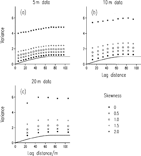
Figure 6.4 shows the experimental variograms for the three sizes of field with
randomly located outliers and for several coefficients of skewness. As the
Figure 6.4 Experimental variograms (shown by point symbols) computed from
simulated fields of various sizes: (a) 1600 points (5-m grid); (b) 400 points (10-m
grid); (c) 100 points (20-m grid), with skewness caused by randomly located outliers. The
solid lines represent the spherical generating function.
116 Reliability of the Experimental Variogram and Nested Sampling