Webster R., Oliver M.A., Geostatistics for Environmental Scientists

Подождите немного. Документ загружается.

Spatial dependence may occur at two distinct scales, and these may be

represented in the variogram as two spatial components. The nested spherical,

or double spherical, function is the one that has been used most often in these

circumstances. Its equation is

gðhÞ¼





()

þc





()

for 0 < h  a

;

þc





()

for a

< h a

;

þc

for h > a

;

ð5:35Þ

where c

and a

are the sill and range of the short-rang e component of the

variation, and c

and a

are the sill and range of the long-ra nge component. If it

appears to need a nugget then that can be added as a third component, and

Figure 5.10(b) shows this combination.

5.4 PERIODICITY

A variogram may seem to ﬂuctuate more or less periodically, rather than increase

monotonically, and we might try to describe it with a periodic function. The

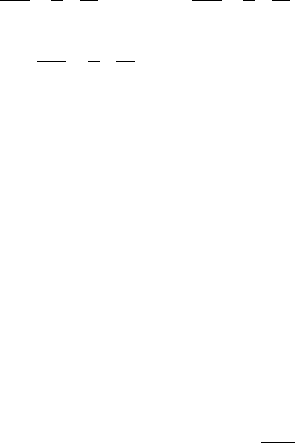
simplest such function is a sine wave, as shown in Figure 5.12(a), with equation

gðhÞ¼W 1  cos

2ph



; ð5:36Þ

where W and v are the amplitude and length of the wave, respectively.

The gradient at the origin is 0, which, as mentioned above, is undesirable.

Usually, however, we ﬁnd that the periodicity is superimposed on some other

source of variation and that the combined model increases from the origin more

steeply. Figure 5.12(b) shows an example of it superimposed on an exponential

function. An example from actual soil survey is illustrated in Chapter 7.

We might be tempted to move the curve along the abscissa to ﬁt the

experimental values so that it increases more nearly linearly from lag 0. We

have drawn such a function as the dashed line in Figure 5.12(a). In other

words, we have introduced a phase shift, f. If we designate the angle 2ph=v as

u for simplicity then the equation becomes

gðhÞ¼Wf1  cosðu  fÞg: ð5:37Þ

Unfortunately, the resulting function is not guaranteed to be CNSD, and so the

temptation should be resisted.

Equation (5.36) is valid for one dimension only; it is not CNSD in R

and R

In two and three dimensions the ﬂuctuation must damp, i.e. become less

Periodicity 97

pronounced with increasing lag distance. Damping can be achieved by division

of the sine or cosine function by a function of the lag distance. Choosing again

the simplest function, we can write

gðhÞ¼W 1 

sinu



; ð5:38Þ

which increases from zero at h ¼ 0, and this appears in Figure 5.12(c).

This model is valid in one, two and three dimensions. Journel and Huijbregts

(1978) show that it has a relative amplitude, which they deﬁne as

b ¼

fmax½gðhÞ  cg; ð5:39Þ

where max½gðhÞ is the maximum semivariance of the function, and c is the

a priori variance, the horizontal line in Figure 5.12(c). In equation (5.38) b is

approximately 0.217, and it occurs where 2:5ph=v  5:6. It is the maximum

for a periodic model in R

Figure 5.12 Periodic and hole effect models: (a) simple sine wave of length 2p (solid)

and with phase shift (dashed line); (b) sine wave superimposed on an exponential

function; (c) damped sine wave of period 2:5p (with maximum marked at h  5:6);

(d) model with Bessel function J

, equation (5.40), with distance parameter set to 10

(giving maximum at h  5:6).

98 Modelling the Variogram

Usually in such cases the damping is such that only the ﬁrst undulation is

substantial. The corresponding covariance function, (see Figure 4.3(f)), appears

to have a single depression in it: it is said to exhibit a hole effect.

Another model that might describe a less pronounced hole effect satisfactorily

embodies the Bessel function J

gðhÞ¼c 1  exp 



2ph



; ð5:40Þ

where J

is the Bessel function of the ﬁrst kind, and v

is a distance parameter

corresponding roughly to wavelength. The maximum is only 0.118 times the

variance of the process. Figure 5.12(d) shows an example in which v

has been

set to 10 to give a maximum at the same lag distance, 5.6, as in the truly

periodic models.

Practitioners should treat wavy experimental variograms with caution. The

experimental values are themselves correlated, the more so as the correlation in

the original data strengthens. One consequence of this is that any underlying

wave-like ﬂuctuation tends to be exaggerated in the esti mates: the wave does

not damp as much as you might expect, even with moderately long runs

(200–300) of data. Before trying to ﬁt a periodic function to such a set of points,

the user sho uld ask what evidence there is of periodicity in the phenomenon

being investigated. If there is none and the apparent periodicity or hole is weak

then do not try to force a periodic model on the variogram. This is a speciﬁc case

of the more general advice that any variogram model should accord with what

you know of the underlying variable, such as the soil, geology, landscape, or

sources of pollution that you are studying.

5.5 ANISOTROPY

Variation can itself vary with direction. If it can be made to seem isotropic by

transformation of the horizontal scales then it is called geometric or afﬁne

anisotropy. Such anisotropy can be taken into account by a simple linear

transformation of the rectangular coordinates. It is perhaps best envisaged for a

process with a spherical variogram in which the range, instead of being a cons-

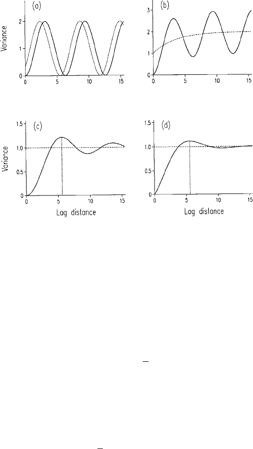
tant, describes an ellipse in the plane of the lag. This is shown in Figure 5.13,

where A is the maximum diameter of the ellipse, i.e. the range in the direction of

greatest continuity (least change with separating distance), and B is the minimum

diameter, perpendicular to the ﬁrst, and is the range in the direction of least

continuity (greatest change with separating distance). The angle ’ is the direction

in which the continuity is greatest. The equation for transformation is then

Vð#Þ¼fA

cos

ð#  ’ÞþB

sin

ð# ’Þg

1=2

; ð5:41Þ

where V deﬁnes the anisotropy, and # is the direction of the lag.

Anisotropy 99

If we insert Vð#Þ into the spherical function then we have

gðh;#Þ¼

3jhj

2Vð#Þ



jhj

Vð#Þ



()

for 0 < jhjVð#Þ;

c for jhj > Vð#Þ:

ð5:42Þ

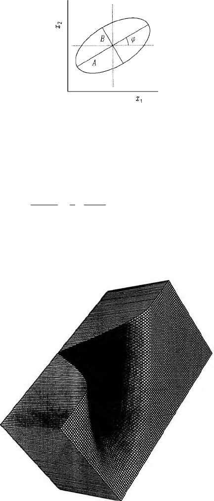
Figure 5.14 shows an example of its surface in two dimensions as a prespective

diagram.

Figure 5.13 A representation of geometric anisotropy in which the ellipse describes the

range of a spherical variogram in two dimensions. The diameter A is the maximum range

of the model, B is the minimum range, and ’ is the direction of the maximum range.

Figure 5.14 Perspective diagram of an anisotropic spherical variogram.

100 Modelling the Variogram

We can derive from equation (5.41) an anisotropy ratio, R ¼ A=B, and it

may be convenient to rewrite equation (5.41) with this replacing B:

Vð#Þ¼ A

cos

ð# ’Þþ



sin

ð#  ’Þ

()

1=2

: ð5:43Þ

This transformation in effect allows the variation to be repr esented in an

isotropic form. It is as if the soil were on a rubber sheet and stretched in the

direction parallel to B until B ¼ A and the ellipse becomes a circle.

The function Vð#Þ can be applied to the power function for unbounded

variation:

gðh;#Þ¼½fA

cos

ð#  ’ÞþB

sin

ð# ’Þg

1=2

jhj

¼½Vð#Þjhj

: ð5:44Þ

Here the roles of A and B are inverted; they are now gradien ts with A, the

larger, being the gradient in the direction of greatest rate of change and B, the

smaller, being the gradient in the direction of the smallest rate.

5.6 FITTING MODELS

The models described above are those that are commonly used for variograms

in resource survey. All are theoretically based. Our task now is to ﬁt them to the

experimental or sample values. One might have thought that after so many

years of geostatistical deve lopment and practice—more than 40 since Matheron

(1965) published his seminal the sis and more than 30 since the ﬁrst textbooks

appeared—that the task would be stra ightforward with standard algorithms

and well-tried software. If so one would be wrong. Choosing models and ﬁtting

them to data remain among the most controversial topics in geostatistics.

There are still practitioners who ﬁt models by eye and who defend their

practice with vigour. They may justify their attitude on the grounds that when

kriging the resulting estimates are much the same for all reasonable models of

the variogram—so why worry about reﬁnement? There are others who ﬁt

models numerically and automatically using ‘black-box’ software, often with-

out any choice, judgement or control. This too can have unfortunate con-

sequences. However, there is controversy among those who ﬁt models

mathematically about which methods to use and by what criteria they should

judge success.

Fitting models is difﬁcult for several reasons, including the following:

(i) the accuracy of the observed semivariances is not constant.

(ii) the variation may be anisotropic.

Fitting Models 101

(iii) the experimental variogram may contain much point-to-point ﬂuctuation.

(iv) most models are non-linear in one or more parameters.

Items (i)–(iii) make ﬁtting by eye unreliable. The ﬁrst two impair one’s intuition,

ﬁrstly because the brain cannot judge the weights to attribute to the semivar-

iances, and secondly because one cannot see the variogram in three dimensions

without constructing a stereogram or physical model, and for three-dimen-

sional variation one needs a fourth dimension. Scatter, item (iii), usually means

that any one of several models might be drawn through the values. It can also

lead to unstable mathematical solutions, and it exacerbates the consequences of

item (iv) because the non-linear parameters must be found by iteration.

Further, at the end one should be able to put standard errors on the estimates

of the parameters.

We also warn against a practice, still common, of choosing the dispersion

variance in a ﬁnite region to estimate the sill of a bounded model for the regional

variogram. For such a region the sill is always greater than the dispersion

variance. Their relation is shown in Figure 4.4. The curve is the variogram of a

second-order stationary process in one dimension of ﬁnite length, as on a

transect. The variogram is extended to the limit of the transect, and in these

circumstances the two shaded portions of the graph should be equal. Clearly the

sill, the a priori variance of the process, must exceed the dispersion variance,

which is estimated by the variance of the data.

We recommend a procedure that embodies both visual inspection and

statistical ﬁtting, as follows. First plot the experimental variogram. Then choose,

from the models listed above, one or more with approximately the right shape

and with sufﬁcient detail to honour the principal trends in the experim ental

values that you wish to represent. Then ﬁt each model in turn by weighted least

squares, i.e. by minimizing the sums of squares, suitably weighted (see below),

between the experimental and ﬁtted values. Finally, inspect the result graphi-

cally by plotting the ﬁtted model on the same pair of axes as the experimental

variogram. Does the ﬁtted function look reasonable? If all the plausible models

seem to ﬁt well you might choose from among them the one with smallest

residual sum of squares or smallest mean square.

The experimental isotropic variogram on the left-hand side of Figure 5.1 was

computed from a fairly small subset of the Broom’s Barn data of 87 sites. It

shows how much point-to-point ﬂuctuation can occur with rather few data (see

Chapter 6), emphasizing the point in item (iii) above. We ﬁtted circular,

spherical, exponential and power functions to these experimental values, and

they appear in that order as the solid lines in the ﬁgure. No one model evidently

ﬁts better than any other, and this impression is supported by the small

differences between the mean squared residuals (MSR) in Table 5.1. The

experimental variogram computed from the full data for Broom’s Barn of 434

sites appears on the right-hand side of the ﬁgure with the same set of functions

ﬁtted. The form of this sequence is simple; it increases smooth ly in a gentle

102 Modelling the Variogram

curve from near the origin and seems to ﬂatten nea r the maximum lag to which

it has been computed. There are much larger differences among the mean

squared residuals in this case because the smooth form of the experimental

variogram enables a much more accurate ﬁt of the model. The spherical

function clearly ﬁts best according to its MSR. The MSRs for the full set of

data are substantially smaller than are those for the subset, except for the power

function. There are also considerable differences among the model parameters

for the two variograms; in particular the nugget varianc es are larger for the

variogram of the subset and the distance parameters are all smaller. These

differences in the estimates of the parameters are important because they carry

through to affect the accuracy of kriged predictions (see Chapter 8).

Never accept a ﬁt without inspecting it afterwards; it might be poor because

(i) you chose an unsuitable model in the ﬁrst place;

(ii) you gave poor estimates of the parameters at the start of the iteration;

(iii) there was lot of scatter in the experimental variogram; or

(iv) the computer program was faulty.

Further, bear in mind the advice above, namely, that the model should accord

with what you know of the region.

Table 5.1 Models ﬁtted to the variogram of log

K at Broom’s Barn Farm for the full

data (434 sites) and a subset of these (87 sites), their parameter values, and the mean

squared residual (MSR). The symbols are as deﬁned in the text.

Model c

ca=mr=mwa MSR

Circular 0.00512 0.01462 386.6 0.000172

(434)

Circular 0.00925 0.01043 362.0 0.000777

(87)

Spherical 0.00466 0.01515 432.0 0.000155

(434)

Spherical 0.00824 0.01136 376.4 0.000774

(87)

Pentaspherical 0.00421 0.01570 514.1 0.000248

(434)

Pentaspherical 0.00757 0.01203 434.0 0.000775

(87)

Exponential 0.00196 0.01973 251.0 0.001054

(434)

Exponential 0.00405 0.01618 130.8 0.000776

(87)

Power function 0 0.00173 0.400 0.003295

(434)

Power function 0 0.00431 0.251 0.000828

(87)

Fitting Models 103

Fitting models in this way is a form of non-linear regression, and you might

think of writing your own program to do it. We recommend that unless you are

proﬁcient in numerical analysis you do not. There are now several well-tried

programs written by professionals that ﬁt models by weighted least squares.

These include GenStat (Payne, 2006) in which the standard models listed above

are already programmed and which is what we use, and SAS (SAS Institute,

1999). The last uses the Levenberg–Marquardt method, which has almost

become a standard for non-linear model ﬁtting (Marquardt, 1963). We give an

example of a GenStat program for ﬁtting non-linear models in Appendix B. If

you do not have access to any of these programs then you might take the code

for the Marquardt algorithm in Fortran from Press et al. (1992). Ratkowsky

(1983) also tackles the subject in a clear and practical way, and the book

includes a suite of subroutines for modelling.

We can call the above approach ‘ﬁt statistically, view afterwards’. Another

approach is the reverse: ‘ﬁt visually, statistics afterwards’. Pannatier (1995)

takes this route with his program Variowin, which is interactive in a Windows

environment. In Variowin you form the experimental variogram from sample

data and you display it on the computer’s screen. You select a plausible model

from those embodied in the program—there are few—and give starting values

for its parame ters from which the machine draws a graph. The program

simultaneously computes a goodness-of-ﬁt criterion, which is a standardized

residual sum of squares. You then adjust the values of the parameters to try to

improve the ﬁt visually, and as you do so the program redraws the model in real

time and recomputes the goodness-of-ﬁt criterion. It also compares the criterion

with the best it has found to date and stores the criterion’s value and the

associated values of the parameters if the new ﬁt is better. You terminate the

ﬁtting when you are satisﬁed with the approximation or no further improve-

ment seems possible. In our experience it works well, though never better than

GenStat (Webster and Oliver, 1997).

5.6.1 What weights?

We mentioned above that the experimental semivariances,

gðhÞ, vary in their

reliability, partly because they are based on varying numbers of paired

comparisons, mðhÞ in equation (4.40), and partly because the conﬁdence in

an estimate of variance decreases as the variance increases. In general, there-

fore, assigning equal weight to all

gðhÞ is unsatisfactory, especially if the mðhÞ

vary widely with changing h. We can take the latter into account simply by

weighting in proportion m. The inverse relation between the reliability of an

estimate of variance and the variance itself led Cressie (1985) to propose a more

elaborate weight at a lag h

in the form

mðh

Þ=g

2

ðh

Þ;

104 Modelling the Variogram

where g

2

ðh

Þ is the value of semivariance predicted by the mod el. McBratney

and Webster (1986) reﬁned this further as

mðh

gðh

Þ=g

3

ðh

Þ;

where

gðh

Þ is the observed value of the semivarian ce at h

. Both of the last two

schemes tend to give more weight at the shorter lags than does weighting on

the numbers of pairs alone, and so the ﬁtting is closer there. This is usually

desirable for kriging (see Chapter 8), though it might be less desirable if the aim

is to estimate the spatial scale of variation.

The process of ﬁtting must iterate even where all the parameters are linear

because the weights in the two schemes depend on the values expected from the

model. Our experience is that in most instances there is little change after the

ﬁrst iter ation, which is therefore enough.

5.6.2 How complex?

Let us return to the question we posed in the beginning of the chapter: how

closely should the model follow the ﬂuctuation in the experimental variogram?

The best simple model, with few parameters, might ﬁt the experimental

variogram poorly, especially if there is much point-to-point scatter. We might

seek a more complex model, therefore, bearing in mind that it is alm ost always

possible to improve the ﬁt in the least-squares sense by increasing the numbers

of parameters, say p. We could continue to increas e p until the model ﬁtted

perfectly, but clearly that is not a sensible answer. We must compromise

between parsimony (few parameters) and close ﬁt (more parameters), and

one way of achieving that is to use Akaike’s (1973) information criterion (AIC):

AIC ¼2lnðmaximized likelihoodÞþ2ðnumber of parametersÞ:

The AIC is estimated by

AIC ¼ n ln



þ n þ 2



þ nlnR þ 2p; ð5:45Þ

where n is the number of points on the variogram, p is the number of

parameters in the model, and R is the mean of the squared residuals between

the experimental values and the ﬁtted model. We may then choose the model

for which

AIC is least. The quantity in braces is constant for any one

experimental variogram, so we need compute only

A ¼ n lnR þ 2 p: ð5:46Þ

Fitting Models 105

Least-squares ﬁtting minimizes R. If, however, R is further diminished only by

increasing p (n is constant) we might discover that

A is increased; we should

have paid an unacceptable penalty for the greater complexity to achieve the

closer ﬁt.

We illustrate the application of the AIC to modelling the variogram of

available copper in the topsoil of the Borders Region of Scotland. The data

are from an original study by McBratney et al. (1982 ). There were some 2000

values from the eastern portion of the Region. They were transformed to their

Figure 5.15 Experimental variogram of log

Cu in the Borders Region of Scotland

with ﬁtted models: (a) single spherical; (b) exponential; (c) double (nested) spherical;

(d) double exponential.

106 Modelling the Variogram