Webster R., Oliver M.A., Geostatistics for Environmental Scientists

Подождите немного. Документ загружается.

research, for they published it in the house journal of their institute, where their

paper lay dormant for many years. The technique had to be rediscovered not

once but several times by, for example, Krumbein and Slack (1956) in geology,

and Hammond et al. (1958) and Webster and Butler (1976) in soil science. We

describe it in Chapter 6.

We next turn to Russia. In the 1930s A. N. Kolmogorov was studying

turbulence in the air and the weather. He wanted to describe the variation and

to predict. He recognized the complexity of the systems with which he was

dealing and found a mathematical descript ion beyond reach. Nowadays we

might call it chaos (Gleick, 1988). However, he also recognized spatial correla-

tion, and he devised his ‘structure function’ to represent it. Further, he worked

out how to use the function plus data to interpo late optimally, i.e. without bias

and with minimum variance (Kolmogorov, 1941); see also Gandin (1965).

Unfortunately, he was unable to use the method for want of a computer in

those days. We now know Kolmog orov’s structure function as the variogram

and his technique for interpolation as kriging. We deal with them in Chapters 4

and 8, respectively.

The 1930s saw major advances in the theory of sampling, and most of the

methods of design-based estimation that we use today were worked out the n

and later presented in standard texts such as Cochran’s Sam pling Techniques,of

which the third edition (Cochran, 1977) is the most recent, and that by Yates,

which appeared in its fourth edition as Yates (1981). Yates’s (1948) investiga-

tion of systematic sampling introduced the semivariance into ﬁeld survey. Von

Neumann (1941) had by then already proposed a test for dependence in time

series based on the mean squares of successive differences, which was later

elaborated by Durbin and Watson (1950) to become the Durbin–Watson

statistic. Neither of these leads were followed up in any concerted way for

spatial analysis, however.

Mate´rn (1960), a Swedish forester, was also concerned with efﬁcient

sampling. He recognized the consequences of spatial correlation. He derived

theoretically from random point processes several of the now familiar functions

for describing spatial covariance, and he sho wed the effects of these on global

estimates. He acknow ledged that these were equivalent to Jowett’s (1955)

‘serial variation function’, which we now know as the variogram, and men-

tioned in passing that Langsaetter (1926) had much earlier used the same way

of expressing spatial variation in Swedish forest surveys.

The 1960s bring us back to mining, and to two men in particular. D. G.

Krige, an engineer in the South African goldﬁelds, had observed that he could

improve his estimates of ore grades in mining blocks if he took into account the

grades in neighbouring blocks. There was an autocorrelation, and he worked

out empirically how to use it to advantage. It became practice in the gold mines.

At the same time G. Matheron, a mathematician in the French mining schools,

had the same concern to provide the best possible estimates of mineral grades

from autocorrelated sample data. He derived solutions to the problem of

A Little History 7

estimation from the fundamental theory of random processes, which in the

context he called the theory of regionalized variables. His doctoral thesis

(Matheron, 1965) was a tour de force.

From mining, geostatistics has spread into several ﬁelds of application,

ﬁrst into petroleum engineering, and then into subjects as diverse as hydro-

geology, meteorology, soil scie nce, agriculture, ﬁsheries, pollution, and envir-

onmental protection. There have been numerous developments in technique,

but Matheron’s thesis remains the theoretical basis of most present-day practice.

1.3 FINDING YOUR WAY

We are soil scientists, and the content of our book is inevitably coloured by our

experience. Nevertheless, in choosing what to include we have been strongly

inﬂuenced by the questions that our students, colleagues and associates have

asked us and not just those techniques that we have found useful in our own

research. We assume that our readers are numerate and familiar with

mathematical notation, but not that they have studied mathematics to an

advanced level or have more than a rudimentary understanding of statistics.

We have structured the book largely in the sequence that a practitioner

would follow in a geostatistical project. We start by assuming that the data are

already available. The ﬁrst task is to summarize them, and Chapter 2 deﬁnes the

basic statistical quantities such as mean, variance and skewness. It describes

frequency distributions, the normal distribution and transformations to stab ilize

the variance. It also introduces the chi-square distribution for variances. Since

sampling design is less important for geostatistical prediction than it is in

classical estimation, we give it less emphasis than in our earlier Statistical

Methods (Webster and Oliver, 1990). Nevertheless, the simpler designs for

sampling in a two-dimensional space are described so that the parameters of

the population in that space can be estimated without bias and with known

variance and conﬁdence. The basic formulae for the estimators, their variances

and conﬁdence limits are given.

The practitioner who knows that he or she will need to compute variograms

or their equivalents, ﬁt models to them, and then use the models to krige can go

straight to Chapters 4, 5, 6 and 8. Then, depending on the circumstances, the

practitioner may go on to kriging in the pres ence of trend and factorial kriging

(Chapter 9), or to cokriging in which additional variables are brought into play

(Chapter 10). Chapter 11 deal s with disjunctive kriging for estimating the

probabilities of exceeding thresholds.

Before that, however, newcomers to the subject are likely to have come

across various methods of spatial interpolation already and to wonder whether

these will serve their purpose. Chapter 3 describes brieﬂy some of the more

popular methods that have been proposed and are still used frequently for

prediction, concentrating on those that can be represented as linear sums of

8 Introduction

data. It makes plain the shortcomings of these methods. Soil scientists are

generally accustomed to soil classiﬁc ation, and they are shown how it can be

combined with classical estimation for prediction. It has the merit of being the

only means of statistical pred iction offered by classical theory. The chapter also

draws attention to its deﬁciencies, namely the quality of the classiﬁcation and

its inability to do more than predict at points and estimate for whole classes.

The need for a different approach from those described in Chapter 3, and the

logic that underpins it, are explained in Cha pter 4. Next, we give a brief

description of regionalized variable theory or the theory of spatial random

processes upon which geostatistics is based. This is followed by descriptions of

how to estimate the variogram from data. The usual computing formula for the

sample variogram, usually attributed to Matheron (1965), is given and also

that to estimate the covariance.

The sample variogram must then be modelled by the choice of a mathema-

tical function that seems to have the right form and then ﬁtting of that function

to the observed values. There is probably not a more contentious topic in

practical geostatistics than this. The common simple models are listed and

illustrated in Chapter 5. The legitimate ones are few because a model variogram

must be such that it cannot lead to negative variances. Greater complexity can

be modelled by a combination of simple models. We recommend that you ﬁt

apparently plausible models by weighted least-squares approximation, graph

the results, and compare them by statistical criteria .

Chapter 6 is in part new. It deals with several matters that affect the

reliability of estimated variograms. It examines the effects of asymmetrically

distributed data and outliers on experimental variograms and recommends

ways of dealing with such situations. The robust variogram esti mators of

Cressie and Hawkins (1980), Dowd (1984) and Genton (1998) are compared

and recommended for data with outliers. The reliability of variograms is also

affected by sample size, and conﬁdence inte rvals on estimates are wider than

many practitioners like to think. We show tha t at least 100–150 sampling

points are needed, distributed fairly evenly over the region of interest. The

distances between sampling points are also important, and the chapter

describes how to design nested surveys to discover economically the spat ial

scales of variation in the absence of any prior inform ation. Residual maximum

likelihood (REML) is introduced to analyse the components of variance for

unbalanced designs, and we compare the results with the usual least-squares

approach.

For data that appear periodic the covariance analysis may be taken a step

further by computation of power spectra. This detour into the spectral domain is

the topi c of Chapter 7.

The reader will now be ready for geostatistical prediction, i.e. kriging.

Chapter 8 gives the equations and their solutions, and guides the reader in

programming them. The equations show how the semivariances from the

modelled variogram are used in geostatistical estimation (kriging). This chapter

Finding Your Way 9

shows how the kriging weights depend on the variogram and the sampling

conﬁguration in relation to the target point or block, how in general only the

nearest data carry signiﬁcant weight, and the practical consequences that this

has for the actual analysis.

A new Chapter 9 pursues two themes. The ﬁrst part describes kriging in the

presence of trend. Means of dealing with this difﬁculty are becoming more

accessible, although still not readily so. The means essentially involve the use of

REML to estimate both the trend and the parameters of the variogram model of

the residuals from the trend. This model is then used for estimation, either

where there is trend in the variable of interest (universal kriging) or where the

variable of interest is correlated with that in an external variable in which there

is trend (kriging with external drift). These can be put into practice by the

empirical best linear unbiased predictor.

Chapter 10 describes how to calculate and model the combined spatial

variation in two or more variables simult aneously and to use the model to

predict one of the variables from it, and others with which it is cross-correlated,

by cokriging.

Chapter 11 tackles another difﬁcult subject, namely disjunctive kriging. The

aim of this method is to esti mate the probabilities, given the data, that true

values of a variable at unsampled places exceed speciﬁed thresholds.

Finally, a completely new Chapter 12 describes the most common methods of

stochastic simulation. Simulation is widely used by some environmental

scientists to examine potential scenarios of spatial variation with or without

conditioning data. It is also a way of determining the likely error on predictions

independently of the effects of the sampling sch eme and of the variogram, both

of which underpin the kriging variances.

In each chapter we have tried to provide sufﬁcient theory to complement

the mechanics of the methods. We then give the formulae, from which you

should be able to program the methods (except for the variogram modelling in

Chapter 5). Then we illustrate the results of applying the methods with

examples from our own experience.

10 Introduction

Basic Statistics

Before focusing on the main topic of this book, geostatistics, we want to ensure

that readers have a sound understanding of the basic quantitative methods for

obtaining and summarizing information on the environment. There are two

aspects to consider: one is the choice of variables and how they are measured;

the other, and more important, is how to sample the environment. This chapter

deals with these. Chapter 3 will then consider how such records can be used for

estimation, prediction and mapping in a classical framew ork.

The environment varies from place to place in almost every aspect. There are

inﬁnitely many places at which we might record what it is like, but practically

we can measure it at only a ﬁnite number by sampling. Equally, there are many

properties by which we can describe the environment, and we must choose

those that are relevant. Our choice might be based on prior knowledge of the

most signiﬁcant descriptors or from a preliminary analysis of data to hand.

2.1 MEASUREMENT AND SUMMARY

The simplest kind of environmental variable is binary, in which there are only

two possible states, such as present or absent, wet or dry, calcareous or non-

calcareous (rock or soil). They may be assigned the values 1 and 0, and they

can be treated as quantitative or numerical data. Other features, such as classes

of soil, soil wetness, stratigraphy, and ecological communities, may be recorded

qualitatively. These qualitative characters can be of two types: unordered and

ranked. The structure of the soil, for example, is an unordered variable and may

be classiﬁed into blocky, granular, platy, etc. Soil wetness classes—dry, moist,

wet—are ranked in that they can be placed in order of increasing wetness. In

both cases the classes may be recorded numerically, but the records should not

be treated as if they were measured in any sense. They can be converted to sets

of binary variables, called ‘indicators’ in geostatistics (see Chapter 11), and can

often be analysed by non-parametric statistical methods.

Geostatistics for Environmental Scientists/2nd Edition R. Webster and M.A. Oliver

# 2007 John Wiley & Sons, Ltd

The most informative records are those for which the variables are measured

fully quantitatively on continuous scales with equal intervals. Examples include

the soil’s thickness, its pH, the cadmium content of rock, and the proportion of

land covered by vegetation. Some such scales have an absolute zero, whereas

for others the zero is arbitrary. Temperature may be recorded in kelvin (absolute

zero) or in degrees Celsius (arbitrary zero). Acidity can be measured by

hydrogen ion concentration (with an absolute zero ) or as its negative logarithm

to base 10, pH, for which the zero is arbitrarily taken as log

1 (in moles per

litre). In most instances we need not distinguish between them. Some properties

are recorde d as counts, e.g. the number of roots in a given volume of soil, the

pollen grains of a given species in a sample from a deposit, the number of plants

of a particular type in an area. Suc h records can be analysed by many of the

methods used for continuous variables if treated with care.

Properties measured on continuous scales are amenable to all kinds of

mathematical operation and to many kinds of statistical analysis. They are

the ones that we concentrate on because they are the most informative, and

they provide the most precise estimates and predictions. The same statistical

treatment can ofte n be applied to binary data, though because the scale is so

coarse the results may be crude and inference from them uncertain. In some

instances a continuous variable is deliberately converted to binary, or to an

‘indicator’ variable, by cutting its scale at some speciﬁc value, as described in

Chapter 11.

Sometimes, environmental variables are recorded on coarse stepped scales in

the ﬁeld because reﬁned measurement is too expensive. Examples include the

percentage of stones in the soil, the root density, and the soil’s strength. The

steps in their scales are not necessarily equal in terms of measured values, but

they are chosen as the best compromise between increments of equal practical

signiﬁcance and those with limits that can be detected consistently. These scales

need to be treated with some caution for analysis, but they can often be treated

as fully quantitative.

Some variables, such as colour hue and longitude, have circular scales. They

may often be treated as linear where only a small part of each scale is used. It is

a different matter when a whole circle or part of it is represented. This occurs

with slope aspect and with orientations of stones in till. Special methods are

needed to summarize and analyse such data (see Mardia and Jupp, 2000), and

we shall not consider them in this book.

2.1.1 Notation

Another feature of environmental data is that they have spatial and temporal

components as well as recorded values, which makes them unique or determi-

nistic (we return to this point in Chapter 4). In representing the data we must

distinguish measurement, location and time. For most classical statistical

12 Basic Statistics

analyses location is irrelevant, but for geostatistics the location must be

speciﬁed. We shall adhere to the following notation as far as possible through-

out this text. Variables are denoted by italics: an upper-case Z for random

variables and lower-case z for a realization, i.e. the actuality, and also for

sample values of the realization. Spatial position, which may be in one, two or

three dimensions, is denoted by bold x. In most instances the space is two-

dimensional, and so x ¼fx

; x

g, signifying the vector of the two spatial

coordinates. Thus ZðxÞ means a random variable Z at place x, and zð xÞ is

the actual value of Z at x. In general, we shall use bold lower-case letters for

vectors and bold capitals for matrices.

We shall use lower-case Greek letters for parameters of populations and eith er

their Latin equivalents or place circumﬂexes (^), commonly called ‘hats’ by

statisticians, over the Greek for their estimates. For example, the standard

deviation of a population will be denoted by s and its estimate by s or

2.1.2 Representing variation

The environ ment varies in almost every aspect, and our ﬁrst task is to describe

that variation.

Frequency distribution: the histogram and box-plot

Any set of measurements may be divided into several classes, and we may count

the number of individuals in each class. For a variable measured on a

continuous scale we divide the measured range into classes of equal width

and count the number of individuals falling into each. The resulting set of

frequencies constitutes the frequency distribution, and its graph (with fre-

quency on the ordinate and the variate values on the abscissa) is the histogram.

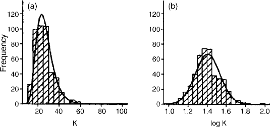
Figures 2.1 and 2.4 are examples. The number of classes chosen depends on the

Figure 2.1 Histograms: (a) exchangeable potassium (K) in mg l

1

; (b) log

K, for the

topsoil at Broom’s Barn Farm. The curves are of the (lognormal) probability density.

Measurement and Summary 13

number of individuals and the spread of values. In general, the fewer the

individuals the fewer the classes needed or justiﬁed for representing them.

Having equal class intervals ensures that the area under each bar is propor-

tional to the frequency of the class. If the class intervals are not equal then the

heights of the bars should be calculated so that the areas of the bars are

proportional to the frequencies.

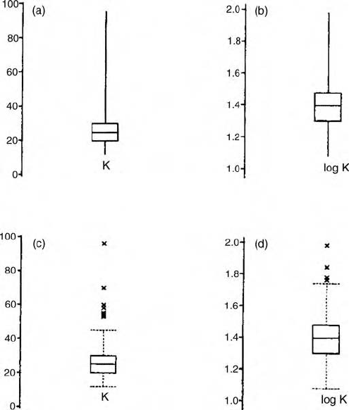
Another popular device for representing a freq uency distribution is the box-

plot. This is due to Tukey (1977). The plain ‘box and whisker’ diagram, like

those in Figure 2.2, has a box enclosing the interquartile range, a line showing

the med ian (see below), and ‘whiskers’ (lines) extending from the limits of the

interquartile range to the extremes of the data, or to some other values such as

the 90th percentiles.

Both the histogram and the box-plot enable us to picture the distribution to

see how it lies about the mean or median and to identify extreme values.

Figure 2.2 Box-plots: (a) exchangeable K; (b) log

K showing the ‘box’ and ‘whiskers’,

and (c) exchangeable K and (d) log

K showing the fences at the quartiles plus and

minus 1.5 times the interquartile range.

14 Basic Statistics

Cumulative distribution

The cumulative distribution of a set of N observations is formed by ordering the

measured values, z

, i ¼ 1; 2; ...; N, from the smallest to the largest, recording

the order, say k, accumulating them, and then plotting k against z. The resulting

graph represents the proportion of values less than z

for all k ¼ 1; 2; ...; N. The

histogram can also be converted to a cumulative frequency diagram, though

such a diagram is less informative because the data are grouped.

The methods of representing frequency distribution are illustra ted in

Figures 2.1–2.6.

2.1.3 The centre

Three quantities are used to represent the ‘centre’ or ‘average’ of a set of

measurements. These are the mean, the median and the mode, and we deal

with them in turn.

Mean

If we have a set of N observations, z

, i ¼ 1; 2; ...; N, then we can com pute their

arithmetic average, denoted by



z,as



z ¼

i¼1

: ð2:1Þ

This, the mean, is the usual measure of central tendency.

The mean takes account of all of the observations, it can be treated

algebraically, and the sample mean is an unbiased estimate of the population

mean. For capacity variables, such as the phosphoru s content in the topsoil of

ﬁelds or daily rainfall at a weat her station, means can be multiplied to obtain

gross values for larger areas or longer periods. Similarly, the mean concentra-

tion of a pollutant metal in the soil can be multiplied by the mass of soil to

obtain a total load in a ﬁeld or catchment. Further, addition or physical mixing

should give the same result as averaging.

Intensity variables are somewhat different. These are quantities such as

barometric pressure and matric suction of the soil. Adding them or multiplying

them does not make sense, but the average is still valuable as a measure of the

centre. Physical mixing will in general not produce the arithmetic average. Some

properties of the environment are not stable in the sense that bodies of material

react with one another if they are mixed. For example, the average pH of a large

volume of soil or lake water after mixing will not be the same as the average of

the separate bodies of the soil or water that you measured previously. Chemical

equilibration takes place. The same can be true for other exchangeable ions.

Measurement and Summary 15

So again, the average of a set of measurements is unlikely to be the same as a

single measurement on a mixture.

Median

The median is the middle value of a set of data when the observations are

ranked from smallest to largest. There are as many values less than the median

as there are greater than it. If a property has been recorded on a coar se scale

then the median is a rough estimate of the true centre. Its principal advantage is

that it unaffected by extreme values, i.e. it is insensitive to outliers, mistaken

records, faulty measurements and exceptional individuals. It is a robust

summary statistic.

Mode

The mode is the most typical value. It implies that the frequency distribution

has a single peak. It is often difﬁcult to determine the numerical value. If in a

histogram the class interval is small then the mid-value of the most frequent

class may be taken as the mode. For a symmetric distribution the mode, the

mean and the median are in principle the same. For an asymmetric one

ðmode  medianÞ2 ðmedian  meanÞ: ð2:2Þ

In asymmetri c distributions, e.g. Figures 2.1(a) and 2.4(a), the median and

mode lie further from the longer tail of the distribution than the mean, and the

median lies between the mode and the mean.

2.1.4 Dispersion

There are several measures for describing the spread of a set of measurements:

the range, interquartile range, mean deviation, stan dard deviation and its

square, the variance. These last two are so much easier to treat mathematically,

and so much more useful therefore, that we concentrate on them almost to the

exclusion of the others.

Variance and standard deviation

The variance of a set of values, which we denote S

, is by deﬁnition

i¼1

ðz



zÞ

: ð2:3Þ

16 Basic Statistics