Webster R., Oliver M.A., Geostatistics for Environmental Scientists
Подождите немного. Документ загружается.


Its disjunctive kriging estimate is obtained by
^
V
DK
½yðx
0
Þy
c
¼Gðy
c
Þþ
X
L
k¼1
1
ffiffiffi
k
p
H
k1
ðy
c
Þgðy
c
Þ
^
H
K
k
fyðx
0
Þg; ð11:44Þ
where L is some small number. The kriged estimates
^
H
K
k
fyðx
0
Þg approach 0
rapidly with increasing k, and so summation need extend over only a few terms
even though the ð1=
ffiffiffi
k
p
ÞH
k1
ðy
c
Þgðy
c
Þ are considerable. Of course, this is the same
as
^
V
DK
½zðx
0
Þz
c
. Conversely, to ob tain the probability of excess we can compute
^
V
DK
½zðx
0
Þ > z
c
¼
^
V
DK
½yðx
0
Þ > y
c
¼ 1 Gðy
c
Þ
X
L
k¼1
1
ffiffiffi
k
p
H
k1
ðy
c
Þgðy
c
Þ
^
H
K
k
fyðx
0
Þg: ð11: 45Þ
11.4.6 Change of support
In describing disjunctive kriging abov e we have treated each target as a ‘point’
with the same support as the data. The simple kriging equations are readily
modified to estimate the Hermite polynomials and hence ZðxÞ over larger blocks
B by replacing the covariances on their right-hand sides with bloc k averages.
The result is a block kriging, i.e. an estimate of the average value of Z within a
target block, say ZðBÞ. It will also produce an estimate of the average
probability that ZðxÞz
c
in B, but note that this probability is not same as
the prob ability that the average of Z in B is less than or equal to z
c
.
As we saw above, in Chapter 4, the distribution of a spatially correlated
variable changes as the support changes. In particular, the variance diminishes
as the support increases and this is evident in the regularized variogram of
Figure 4.7. If we are to estimate the conditional probabilities that block
averages exceed z
c
then we need to take into account the larger support and
to model the change of support. Webster (1991) summarizes the theory and
illustrates it with an example from agricultural science, and Rivoira rd (1994)
treats it more didactically, again with an illustration using the same data. The
subject is beyond the scope of this book , but you can read about the theory and
technique in the two works cited.
11.5 CASE STUDY
To illustrate the method and to enable the results of disjunctive kriging to be
compared with those of ordinary kriging in Chapter 8, we use the data on
exchangeable pota ssium from the soil survey of Broom’s Barn Farm. Chapter 2
Case Study 257

describes them in full, and here we repeat only the most salient features.
Table 11.1 summarizes the statistics of the data and the transforms to standard
normal deviates using Hermite polynomials. It includes the summary for the
common logarithms for comparison.
Figure 11.2 shows the general nature of the problem. Figure 11.2(a) is the
cumulative distribution of exchangeable K as observed. For a defined threshold
concentration, z
c
, we should like to know its equivalent on the standard normal
curve, because then we can calculate confidence limits. We suppose for illustra-
tion that it is 20 mg l
1
of soil. From Figure 11.2(a) we see that the cumulative
sum is approximately 0.24. Tracing this value across by the horizontal dashed
lines to the standard normal distribution on Figure 11.2(b), we see that its
equivalent normal deviate is 0:69, shown by the vertical dashed line there. The
first task therefore is to transform the data to a standard normal distribution so
that we have the equivalences for all reasonable values of z.
The distribution on the original scale (mg l
1
) is strongly skewed, g
1
¼ 2:04
(Figure 11.3(a) and Table 11.1). Taking logarithms removes most of the
skewness, with g
1
¼ 0:39, as shown in Figure 2.1(b).
Figure 11.2 The cumulative distribution: (a) of potassium; (b) of a standard normal
distribution. The vertical dashed line in (a) is for a threshold of 20 mg l
1
, and the others
show how it equates in (b); see text.
Table 11.1 Summary statistics.
Hermite-
Statistic K log
10
K transformed K
Mean 26.3 1.40 0.0740
Median 25.0 1.40 0.104
Standard deviation 9.04 0.134 0.974
Variance 81.706 0.018 00 0.9495
Skewness 2.04 0.39 0.03
Kurtosis 9.45 0.57 0.07
Deficiency threshold 25.0 1.40 0.104
258 Disjunctive Kriging
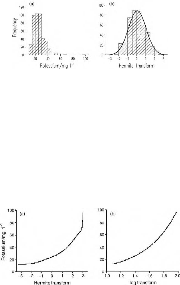
Transforming with Hermite polynomials up to order 7 is more effective,
giving approximate standard normal deviates. The mean and variance depart
somewhat from 0 and 1, respectively. The skewness is virtually nil (0:03), as
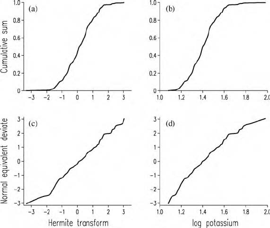
is the kurtosis (0.07), see Figure 11.3(b) and Table 11.1. Figure 11.4(a) shows
the transform function with the measured values plotted against the Hermite
transformed ones. The graph is concave upwards, resulting from the positive
skewness of the data. For a normal distribution the transform function would
be a straight line; the departure from this is a measure of the non-normality. We
show the logarithmic transformation function in Figure 11.4(b) for comparison.
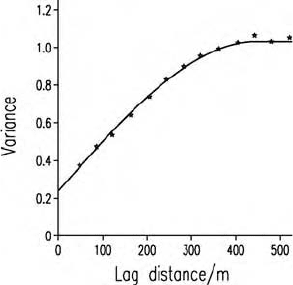
Figure 11.5 shows other features of the transformation , again with those of
the logarithms alongside for comparison. In Figure 11.5(a) and (b) are the
cumulative distributions with GðyÞ plotted against y, the transformed values.
Both are cha racteristically sigmoid, as expected for data from a normal
distribution. In Figure 11.5(c) and (d) we have plotted the normal equivalent
deviates of the cumulative distributions against y. The normal equivalent
Figure 11.3 Histograms of potassium: (a) as measured in mg l
1
; (b) after transforma-
tion by Hermite polynomials with the curve of the normal distribution fitted.
Figure 11.4 Transform functions of potassium at Broom’s Barn Farm: (a) for Hermite
polynomials; (b) for logarithms.
Case Study 259
deviate is the area beneath a curve of the standard normal pdf from 1 to gðyÞ,
equivalent to GðyÞ. For a normal distribution this function plots as a straight
line. For the Hermite transformation of potassium it is straight, apart from local
fluctuation. For the logarithms, however, there is still detectable curvature.
We mentioned above our assumption that zðxÞ is the outcome of a Gaussian
diffusion process for which the cross-variograms of the indicators should be
more structured than the autovariograms. To check that the exchangeable K
conforms we computed the relevant variograms for K > K
c
for c ¼ 20; 25 and
30 mg l
1
, which correspond closely to the quartiles of the cumulative distribu-
tion; they are the cumulants 0.24, 0.51 and 0.75, respectively. The results are
shown in Figure 11.1 with the autoindicator variograms on the left and the
cross-indicator variograms on the right. We have not fitted models to them, but
quite evidently the latter are more structured; any curve fitted closely to the
experimental values will project on to the ordinate near the origin, whereas all
three autovariograms will have substantial nugget variances.
We computed the experimental variogram from the Hermite-transformed
values and fitted an isotropic spherical model to it:
^
gðhÞ¼0:216 þ 0:784 sphð434Þ; ð11:46Þ
Figure 11.5 Cumulative distributions of potassium at Broom’s Barn Farm: (a) the
cumulative sum for the Hermite transform, and (b) for the logarithms; (c) and (d) the
cumulants plotted as normal equivalent deviates.
260 Disjunctive Kriging
in which sphð434Þ indicates the spherical function with a range of 434 m.
Figure 11.6 shows the experimental values as points and the fitted model as a
solid line. Using this model and the transformed values, we estimated the
concentrations of potassium at the nodes of a square grid at 10-m intervals by
punctual kriging of the Hermite polynomials, as described above.
For cereal crops at the time the survey was made, a critical value for readily
exchangeable potassium was 25 mg l
1
; this was the threshold below which the
Ministry of Agriculture, Fisheries and Food (1986) recommended farmers to
fertilize cereal crops. We computed the conditiona l probabilities of the values’
being less than or equal to this threshold at the same grid nodes.
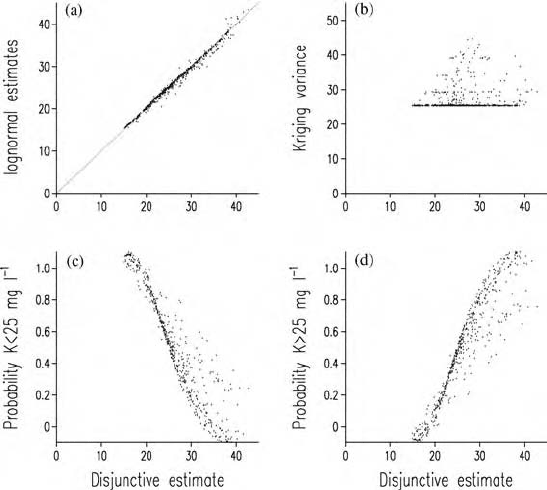
Figure 11.7 is the map of the disjunctively krig ed estimates of exchangeable
K. As it happens in this instance, it is little diff erent from the map made by
lognormal kriging (Figure 8.22), because the transform functions are similar.
We can see this by plotting the disjunctively and lognormally kriged estimates
against each other, as in Figure 11.8(a). There is little scatter in the points from
the solid line of perfect correlation on the graph, and the correlation is
r ¼ 0:994. Figure 11. 8(b) is the scatter diagram of the disjunctively kriged
estimates plotted against the kriging variance. This shows clearly the effect of
the nugget variance in punctual kriging. The nugget variance sets a lower
limited to the precision of the estimates, and this is evident in the horizontal line
at a kriging variance of about 25 (mg l
1
)
2
.
In addition, disjunctive kriging enables us to map the estimated conditional
probabilities of deficiency or excess from the same set of target points. Figures
11.9(a) and 11.9(b) are maps of the probabilities for thresholds of 25 mg l
1
and 20 mg l
1
, respectively.
In Figu re 11.8(c) we hav e plotted the conditional probabilities that the
exchangeable K 25 mg l
1
against the disjunctively kriged estimates. It is
evident from this graph that some of the estimates exceeding the threshold have
Figure 11.6 Variogram of potassium after transformation by Hermite polynomials.
Case Study 261

associated with them fairly large probabilities of deficiency; evidently
we should not judge the likelihood of deficiency from the estimates alone.
You may also notice that some of the points on the graph lie outside the
bounds of 0 and 1 for the probabilities. This is because they are themselves
estimates.
In environmental management we are often concerned with the probabilities
that som e substance exceeds a threshold. If potassium were a pollutant then we
might plot the probabilities of its exceeding the threshold of 25 mg l
1
.We
should then obtain Figure 11.8(d), the inverse of Figure 11.8(c).
In a situation concerning deficiency the farmer would fertilize where the map
showed exchangeable K to be less than 25 mg l
1
, the pale grey and white areas
of Figure 11.7. However, the farmer would not want to risk losing yield where
the estimated concentration of K is more than the threshold and the probability
of deficiency is moderate. If he were prepared to set the maximum risk at a
probability of 0.3 then he should fertilize the areas in Figure 11.9(a) where the
probability is greater, i.e. areas of medium and dark grey and black. The area is
considerable. When the map of probabilities is compared with that of the
estimates it is clear that the farmer could risk loss of yield by taking the
Figure 11.7 Map of exchangeable potassium at Broom’s Barn Farm, estimated by
disjunctive kriging.
262 Disjunctive Kriging
estimates at face value—the area requiring fertilizer is considerably greater
than that where K 25 mg l
1
.
11.6 OTHER CASE STUDIES
Wood et al. (1990) described an application of disjunctive kriging to estimating
the salinity of the soil in the Bet Shean Valley to the west of the River Jordan in
Israel. The combination of climate, irrigation and smectite clay soil has
resulted in significant concentrations of sodium salts in the topsoil. In general,
salinity limits the range of crops that can be grown as well as reducing the
yields of those that can tolerate it. A critical threshold, z
c
,ofelectrical
conductivity (EC) is 4 mS cm
1
: it is w idely rec ogniz ed as marking the onset
of salinization of the soil. The principal crops that are affected by too much salt
in the valley are lucerne, wheat and dates. The losses of yield of lucerne and
dates become serious when this threshold is exceeded. Winter wheat, however,
will still grow, but when the threshold is exceeded it germinates poorly.
Figure 11.8 Scatter of: (a) disjunctively kriged estimates against lognormally kriged
ones; (b) estimates obtained by disjunctive kriging against their estimation variances;
(c) estimated probabilities of deficiency ( 25 mg l
1
) against estimates; (d) estimated
probabilities of excess (> 25 mg l
1
) against estimates.
Other Case Studies 263

Figure 11.9 Maps of probabilities of potassium deficiency at Broom’s Barn Farm with
thresholds of (a) 25 mg l
1
; (b) 20 mg l
1
.
264 Disjunctive Kriging
The EC of the soil solution in November before the onset of winter rain is the
most telling, and it was measured at some 200 points in a part of the valley at
that time to indicate salinity. The EC was then estimated at the nodes of a fine
grid and mapped. The conditional probabilities of the ECs exceeding 4 mS cm
1
were also determined and mapped, and in the event they exceeded 0.3 over
most of the region. There was a moderate risk of salinity in most of the region.
Farmers would find it too costly to remediate the entire area, but they cou ld use
the map of probabilities as a guide for deciding on the priority of areas for
remediation.
Webster a nd Oliver (1 989), Webster and Ri voirar d (1991) and Webster
(1994) used the data from the original survey by McBratney et al. (1982)
of copper and cobalt in the soil of southeast Scotland to study the merit and
relevance of disjunctive kriging in agriculture. Deficiencies of copper
and cobalt in the soil of the region caus e poor health in gr azing sheep and
cattle there. The critical value, z
c
, for copper in the soil is 1 mg kg
1
and for
cobalt 0.25 mg kg
1
. Data from some 3500 sampling points were available,
and from them they computed the probabilities of the soil’s being deficient in
the two trace metals by disjunctive kriging. The concentration of copper
exceeded the 1 mg kg
1
threshold alm ost e verywh ere. The concentratio n is
near t o t he threshol d in only smal l p arts of the reg ion where the estimated
probability of deficiency was typically in the range 0.2–0.3. For cobalt,
however, for w hich the mean c oncentr ation wa s almost e xactly equal to
the threshold of 0.25 mg kg
1
, the estimates for approximately half the
region w ere less than the thres hold with an estimated probability
of deficiency greater than 0.5, and elsewhere most of the computed
probabilities exceeded 0.2. The potential loss of thrift in the animals and
therefore profit to the farmer is considerable, whereas preventive measures
such as suppl ementar y cobalt in the animals ’ fee d or addi tion s in the
fertilizer are cheap. In these circumstance s the farm er would be advised to
take one of these courses of action where the probability of deficiency
exceeded 0.2.
Maps of probabilities also help environmental scientists to design pro-
grammes of remediation for areas considered to be polluted. Once the users
have decided what risks they are prepared to take, the scientist can use such
maps to recommend suitable action. If there are strictly limited funds for
remediation the map of probabilities enables them to assign priorities for
action; the parts of the region where the probabilities are greatest can be
tackled first.
Von Steiger et al. (1996) estimated the concentrations of heavy metals in
polluted soil in part of northeast Switzerland by disjunctive kriging. The
soil contained lead in excess of the Swiss Federal Guide value of 50 mg kg
1
.
The probabilities exceeded 0.3 to the north and east of the town of
Weinfelden, sug gesting that the se areas should be monitored to ensure
that the burden in the soil does not exceed the existing concentrations.
Other Case Studies 265
11.7 SUMMARY
The principles described in this chapter can be applied to various substances
in the environment, whether they are nutrients that might be deficient or
heavy metals and xenobiotics, excesses of whi ch are toxic. The probabilities
of exceeding specific thresholds enable the risk of inaction to be assessed
quantitatively. Disjunctive kriging, in particular, provides environmenta l ana-
lysts with a useful decision-making tool, especially where failure to act could
result in litigation, damage to health or loss of revenue. Assessing this risk is
now feas ible in an optimal way.
266 Disjunctive Kriging