Webster R., Oliver M.A., Geostatistics for Environmental Scientists
Подождите немного. Документ загружается.

the common three-dimensional functions such as the spherical and exponential
models. Finding the correct one-dimensional functions corresponding to them
in two dimensions, C
2
ðhÞ, turns out to be much more complex. This is
presumably why most software packages do not include the turning ban ds
method for R
2
. Even more worrying is that some of those that do include the
method produce patterns of values in which the bands are plainly evident; see,
for example, Figure V.8 on page 148 in Deutsch and Journel (1998). Such
results are unacceptable.
Partly for the above reasons and partly because sequential Gaussian simula-
tion and simulated anneal ing have proved so successful, the turning bands
method has lost favour. We do not devote further attention to it therefore.
Olea (1999) provides a detailed expose´ of the method for those who are
interested.
12.3.5 Algorithms
The above algorithms are expanded with proofs in Olea (1999). Goovaerts
(1997) also describes them and illustrates their application with the data of
Atteia et al. (1994) on soil of the Swiss Jura. The LU decomposition can be
programmed readily in GenStat, MATLAB and S-Plus, for example, alth ough it
is also available in GSLIB (Deutsch and Journel, 1998), as are sequential
Gaussian simulation and simulated annealing. The turning bands method
was in the first edition only of GSLIB (Deutsch and Journel, 1992) and it is
for three dimensions in that library.
12.4 USES OF SIMULATED FIELDS
As above, simulation is not a substitute for estimation; that is not its purpose.
What it does do is give us picture s of the variation to expect between sampling
points as distinct from the smoothed form provided by kriging. By conditioning
the simulation on data we ensure that the fields generated do not stray far from
reality.
Unconditional and conditional sim ulation can give us dense fields of values
on which we can study dispersion and sampling fluctuation, and from which
we can construct confidence intervals on estimates of the variogram, as in the
examples in Chapter 5.
We have already mentioned that repeated simulations enable us to judge the
probability that a variable exceeds a threshold at two or more places in a
neighbourhood. This is valuable for the delimitation of zon es of pollution (for
examples, see Goovaerts, 1997; Fabbri and Trevisani, 2005) and for estimating
the travel time of water and solute through an aquifer which depends on the
joint distribution of transmittivities (see Gotway, 1994).
Uses of Simulated Fields 277
12.5 ILLUSTRATION
Figures 5.5 and 5.6 are examples of random fields produced by unconditional
simulation. We illustrate the results of conditioning by returning to the case
study at Broom’s Barn Farm.
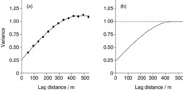
The potassium data for Broom’s Barn Farm were transformed first to normal
scores and the variogram computed on the transformed values. A spherical
function fitted the experimental values with c
0
¼ 0:2536, c ¼ 0:8410 and
a ¼ 458 m; it is shown in Figure 12.1(a). The GSLIB (Deutsch and Journel,
1998) simulation program assumes that the sill variance of the normal score
transform will be unity, and so the above model parameters were adjusted
proportionately to c
0
¼ 0:2326 and c ¼ 0:7674 to ensure this; see
Figure 12.1(b). The latter was used to generate values by sequential Gaussian
simulation on a 10 m 10 m grid with the normal scores of K at 40-m
intervals. Eight simulations were done with a unique random number seed
each time, and the simulated normal scores were transformed back to the
original scales. Their means and variances were calculated (Table 12.1), and
are close to those of the data. Figure 12.2 shows the maps of the eight fields.
There are differences in the local detail, but they reflect the general pattern of
variation shown in Figure 8.22. In particular, there is more local variation in
the maps of the simulated fields than in the kriged maps. Figure 12.3 shows the
corresponding experimental variograms plotted as points at 40-m intervals.
There are small differences among them for the individual fields, but all lie close
to the generating function. We fitted spherical functions to each individually,
Figure 12.1 (a) Experimental variogram of the normal scores of K at Broom’s Barn
and the fitted function; (b) the variogram rescaled to a sill of 1 and used for the sequential
Gaussian simulation.
278 Stochastic Simulation
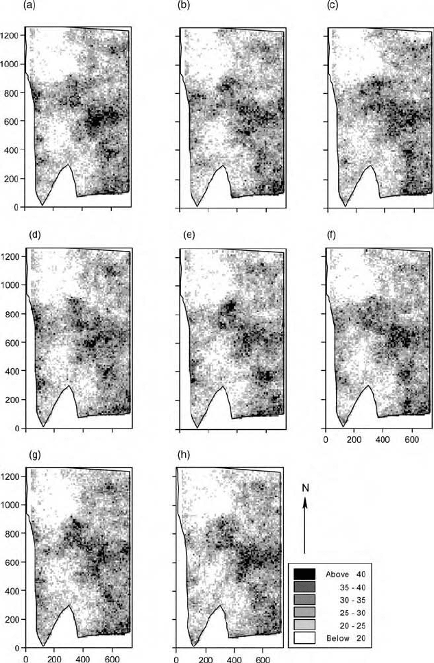
Figure 12.2 Maps of eight fields of values produced by sequential Gaussian simulation
for K at Broom’s Barn.
Illustration 279
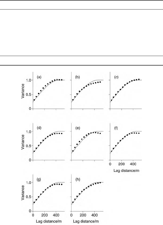
Figure 12.3 Experimental variograms for the eight sequential Gaussian simulated
fields plotted as points with the generating variogram shown in Figure 12.5(b) added to
each as the solid line.
Table 12.1 Means, variances and standard deviations for eight fields simulated by
sequentialGaussiansimulation conditioned by thepotassium datafrom Broom’s BarnFarm.
Simulation Mean Variance Standard deviation
1 25.56 70.76 8.412
2 26.25 62.13 7.882
3 26.27 68.81 8.295
4 26.43 59.34 7.703
5 25.91 63.79 7.987
6 26.33 61.96 7.872
7 26.50 59.85 7.736
8 25.74 58.94 7.677
Raw data 26.31 81.71 9.039
280 Stochastic Simulation

and Table 12.2 gives their model parameters. There are small differences in the
nugget variances, but somewhat larger differences in the ranges from the
generating function.
We also illustrate results using simulated annealing on the same grid and
conditioned on the same normal scor es of K. Figure 12.4 shows the stages in
the annealing process. The first map, Figure 12.4(a), includes the data and
additional values draw n from a normal distribution with the same mean and
variance as the data. The field appears to lack any pattern, and its experimental
variogram, shown in Figure 12.5(a), is effectively flat. The objective function at
this stage, the beginning, is 1. Figure 12.4(b) shows the results after 65 000
swaps, at which stage the objective function had decreased from 1 to 0.5289. A
broad pattern is beginning to develop and is just detectable. The variogram of
the field, presented in Figure 12.5(b), shows only weak structure at this stage,
which manifests itself as long-range autocorrelation. The experimental vario-
gram is still fairly flat near the ordinate, however. After approximately 190 000
swaps the objective function reached 0.0004, and the experimental variogram
is close to the theoretical curve, as is apparent in Figure 12.5(c). The main
features of the spatial pattern are evident in Figure 12.4(c), and this map
resembles those from sequen tial Gaussian simulation (Figure 12.2) with the
same broad features as those from block kriging (Figure 8.22). Nevertheless, it
is not as similar to the latter as are those in Figure 12.2. The maps in Figure
12.4(d) and (e) are for two more simulations that converged after some
195 000 swaps and an objective function of 0.0002. Figure 12.5(d) and (e)
shows their variograms.
The maps in Figure 12(c)–(e) are clearly different from one another and seem
to vary more than do those for sequential Gaussian simulation; there are more
Table 12.2 Model parameters for the spherical function fitted to experimental
variograms from eight fields simulated by sequential Gaussian simulation conditioned by
the potassium data standardized to mean 0 and variance 1 from Broom’s Barn Farm.
Simulation c
0
ca/m Residual Mean Square
1 0.2660 0.7406 412.7 48.68
2 0.2942 0.6209 420.0 227.7
3 0.2546 0.7578 459.6 43.11
4 0.2618 0.6588 395.6 44.80
5 0.2691 0.6744 364.3 151.5
6 0.2635 0.6966 418.8 60.05
7 0.2523 0.6840 409.3 12.01
8 0.2899 0.6818 455.2 186.0
Generator 0.2536 0.8410 454.0
Illustration 281
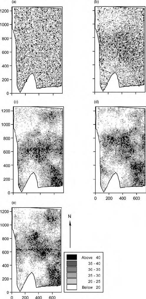
Figure 12.4 Stages in the annealing process: (a) the data plus additional values drawn
from a normal distribution; (b) the result after 65 000 swaps; (c), (d) and (e) the results
after some 190 000 swaps and convergence of the experimental variogram to the
generator, Figure 12.1(a).
282 Stochastic Simulation

differences among them in the detail. Clearly, they all show more local detail
than appears in the kriged map.
Figure 12.5 Experimental variograms of the fields from the simulated annealing in
Figure 12.4: (a) of the initial field; (b) after 65 000 swaps; (c), (d) and (e) after
convergence with some 190 000 swaps. The solid line in each graph is the variogram,
shown in Figure 12.1(a), of the function to which the annealing converges.
Illustration 283

Appendix A
Aide-me´moire for
Spatial Analysis
A.1 INTRODUCTION
This appendix summarizes the steps that a scientist should take in a geostatis-
tical analysis of survey data, beginning with error detection, summary statistics,
exploratory data analysis, the variogram and its modelling, kriging, and
mapping. In many instances data from remote imaging require the same
treatment, and where that is so we mention it.
A.2 NOTATION
The notation is the same as used in the main text, but we repeat it here for
completeness. The geographic coordinates of the sampling points and target
points for prediction are denoted x
1
for eastings (or across the map from left to
right) and x
2
for northings (or from bottom to top on the map). The pair
fx
1
; x
2
g are given the sym bol x in vector notation. The variates are denoted
z
1
; z
2
; ...; and the measured values are denoted zðx
i
Þ for i ¼ 1; 2; ..., for any
one variate.
A.3 SCREENING
Few large files of data are free of mistakes caused by instrumental malfunction
and human error. When you receive data, whether from the field or laboratory
or from remote scanners, check for such mistakes.
Position. Examine the positions of the data in relation to the bounds of the
region. Plot them on a map, known as a ‘posting’.
Geostatistics for Environmental Scientists/2nd Edition R. Webster and M.A. Oliver
# 2007 John Wiley & Sons, Ltd
Do all the points lie within the region?
Are there sampling points in the sea when they should be on the land? If so
why?
Have the coordinates been reversed inadvertently so that northings precede
eastings, i.e. the x
2
precede the x
1
?
Do the points approximately fill the region?
Are the coordinates properly scaled?
Measurements. Screen the measured values, zðx
1
Þ; zðx
2
Þ; .... Pass them
through a program that compares each value in the file against the minimum
and maximum possilbe of the scale and flags any that lie outside these bounds.
Print out the minimum and maximum for each z and check that they are
sensible.
A.4 HISTOGRAM AND SUMMARY
For each variate compute a histogram and plot it, ensuring that all classes are of
the same width. Examine it for outliers, i.e. individuals or small groups that are
isolated from the main body of data. In addition, if you prefer box-plots,
compute them for the zs, to show outliers.
Outliers. If there are outliers identify the ir positions on the map.
Are the y mistakes? If not, what do they repr esent?
Are the y part of the ‘target population’?
If not (e.g. water when you are interested only in land) then replace the
recorded values by a symbol to indicate missing or not applicable.
The statistical treatment of outliers is a complex subject, and if you wish to
retain outliers in your analysis then consult a statistician.
Frequency distribution. Study the shape of the histogram.
Has it more than one peak?
If so, the scene or region almost certainly contains at least two distinct
populations, e.g. lan d and water, farmland and forest.
Is the distribution symmetric?
If it is skewed is the longer tail towards the small values or towa rds the
large?
Summary. Summarize the statistics for each variate by computing:
the number of sampling points and the number of valid values;
the minim um and maximum;
the mea n;
286 Aide-me´moire for Spatial Analysis