Teodorescu P.P. Mechanical Systems, Classical Models Volume I: Particle Mechanics

Подождите немного. Документ загружается.

Problems of dynamics of the particle

451

we find thus again the equations (6.2.29), the latter ones being deduced in the

hypothesis of a uniform motion. In this last case (we have

/2 constTmv== too),

we may write

(

)

222

vgqqgqqvv

αα

αβ β αβ β

′′ ′′

== = =

what was to be expected, because

1gqq

αβ β

′

represents a first integral of the system

of equations (7.2.19'''), where one of these equations may be replaced by the respective

first integral.

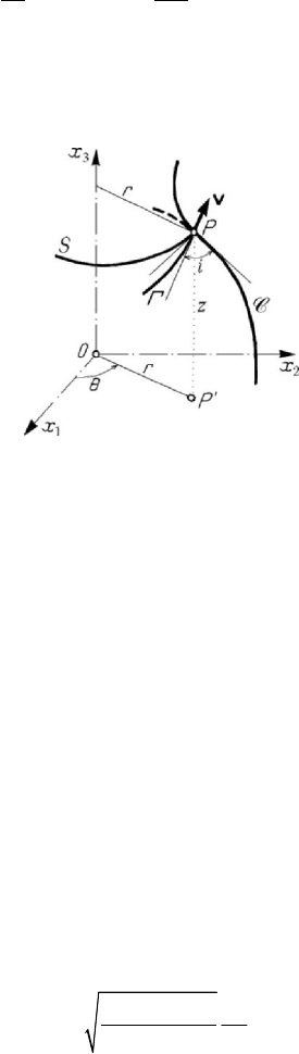
Figure 7.19. Motion of a particle on a geodesic curve of a surface of rotation.

Let us consider, in particular, the case in which the surface

S is a surface of rotation

of parametric equations

cosxrθ

sinxrθ

()xz rϕ

= , where ,,rzθ are

cylindrical co-ordinates (Fig.7.19); in this case,

(

)

22222

d1 d dsrrϕθ

′

=+ +

d/drϕϕ

′

. In the case of a uniform motion

222

ddsvt= , obtaining thus the first

integral

(

)

22 22 2

1constrr vϕθ

′

++==



;

(7.2.20)

we notice that the support of the constraint force passes through the rotation axis, so

that a first integral of areas for the projection

′

of the particle P on the plane

Ox x

reads

constrr Cθθ===



(7.2.20')

The solution of the problem is thus reduced to quadratures. Eliminating the time

between the two first integrals, we obtain

(

)

2222 422

1ddd/rr r kϕθθ

′

++=

222

/kCv= , so that the equation of the geodesic curves passing through the point

(

000 0

,, ()rz rθϕ

) is given by

[]

1()

ϕρ

θθ

′

−

∫

;

(7.2.21)

MECHANICAL SYSTEMS, CLASSICAL MODELS

452

the constant

k of the family of geodesic lines is determined imposing the condition that

the respective line passes through a second given point. If the geodesic curve

Γ pierces

the meridian

C of the point P by an incidence angle i , then the components of the

velocity

v along the meridian and the parallel of the point are cosvi and sinvi,

respectively. The moment of the velocity

v with respect to the axis of rotation

will be equal to

C (corresponding to the first integral of areas) and is given only by the

component

sinvi with the arm level r (Fig.7.19); it results that sinrv i C= . Because

vv= , one obtains Clairaut’s formula

sinrik

, (7.2.22)

where

k is the constant of the family of geodesic lines (the ratio of the constants of the

two first integrals). Reciprocally, if the relation (7.2.22) takes place for all the points of

a curve on a surface, then that one is a geodesic line or a parallel of the surface of

rotation.

2.2 Other applications

In what follows, some particular cases of motion of a particle will be presented, e.g.,

the motion of a particle on a circular helix; as well, some particular methods to solve

problems of dynamics of the particle are considered, for instance the method of

transformation of motions.

2.2.1 Motion of a particle on a circular helix

Let be a heavy particle, constrained to move on a circular helix of parametric

equations

cosxRθ= ,

sinxRθ

/2 tanxp Rθπ θ α

= , where p is the

pitch of the helix, while

α is the angle made by the helix with a horizontal parallel of

the circular cylinder, of radius

R , on which the helix is enveloped (see Chap. 5,

Subsec. 1.3.3, Fig.5.9); in general, we assume that the motion takes place in a resistent

medium, characterized by a viscous resistance

vλ , 0λ > . Euler’s equations of motion

read

mv F v

λ=−



νν

=+, 0 FR

ββ

+ .

If the initial velocity

v is directed so that 0θ



(the particle “moves down” on the

helix), then we have

12 3

cos (sin cos ) sinαθ θ α=−−ii iτ ,

cos sinθθ

−−ii

12 3

sin (sin cos ) cosαθ θ α=− − −ii iβ .

so that, for the given force

Fg we get the components

sinFmg

α= , 0F

, cosFmg

− .

Problems of dynamics of the particle

453

The equation of projection along the tangent leads to

()

sin 1

−

=−, k

= ,

(7.2.23)

where we have put the initial condition (0) 0v

. But /cosvRθα=−



, so that we

obtain (

(0)tanRhθα= )

()

sin 2

tan

kt e

−

=+ −−.

(7.2.23')

In particular, in the case of falling in vacuum (

0λ

, hence 0k

), we develop

into series the exponential function, obtaining

sinvgt α= ,

sin 2

tan 4

hgt

=−

(7.2.23'')

The other two intrinsic equations give the components of the constraint force.

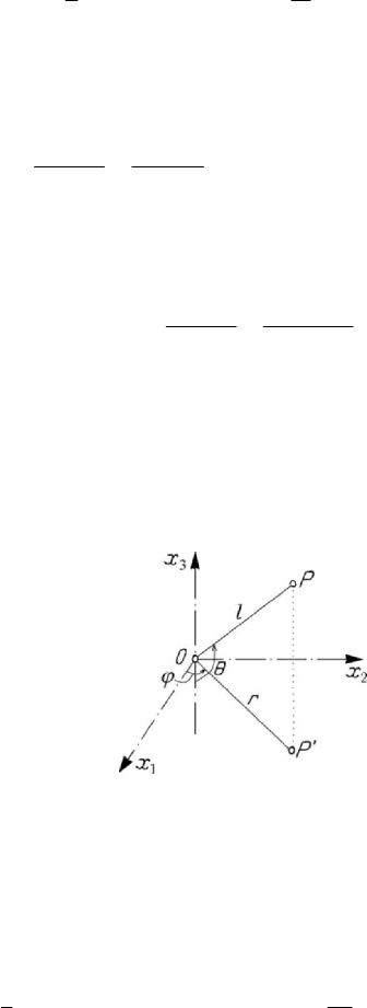
2.2.2 The simple pendulum in a motion of rotation

Let us suppose that the vertical circle on which moves a heavy particle (in particular,

the simple pendulum considered in Subsec. 1.3.1) is rotating with a constant angular

velocity

ω around its vertical diameter. The co-ordinates of the particle are

Figure 7.20. Simple pendulum in a motion of rotation.

sin cosxl tθω= ,

cos sinxl tθω

cosxlθ

− ,

where the applicate

x is directed towards the local ascendent vertical (Fig.7.20).

Because the constraint is rheonomic, we use Lagrange’s equation (6.2.21), where

()

22 2 2

sin

Tmlθω θ=+



sin

Qm mgl θ

=⋅=−

;

we obtain thus

MECHANICAL SYSTEMS, CLASSICAL MODELS

454

sin cos sin 0

θω θ θ θ−+=



(7.2.24)

Introducing the non-dimensional variable

tϕω

, we also may write this equation

in the form (

ddtϕω= , d/dθθϕ

′

)

(cos )sinθθλθ

′′

=− ,

;

(7.2.24')

multiplying by

2θ



and integrating, one obtains the first integral

(

)

sin 2 cos constθθλθ−+ =



(7.2.24'')

the equation

()θθϕ= of the trajectory being thus obtained by a quadrature.

The above considerations are valid for pendulary motions as well as for circular

ones.

2.2.3 Transformation of motions

We – often – have seen that in the study of a motion one may use the results obtained

for other simpler motions. For instance, we have seen that the study of arbitrary

tautochronous motions is reduced to the study of rectilinear tautochronous motions; that

is, in fact, a transformation of motions.

In Subsec. 2.1.5, an interesting analogy between the equilibrium of a perfectly

flexible, torsionable and inextensible thread and a motion of a particle on a

brachistochrone has been stated; that one may be considered as a transformation of

motion too.

The motion of a particle on a smooth surface may be studied by means of the

equations (6.2.24) with respect to Darboux’s trihedron. Let us deform the surface,

assuming that this is possible, so that the lengths of the lines drawn on the surface do

remain invariable; in such a transformation, also the geodesic curvatures remain

invariant. Let us modify the force

F so that its projection on the plane tangent to the

surface (hence, the components

and

F ) do remain unchanged; in this case, the first

and the third equation (6.2.24) which specify the motion remain – further – valid, and

the motion is the same as in the first case (the study of this new motion may be much

more simple); obviously, the constraint force given by the second equation (6.2.24) is

another one. In the case of a developable surface, the problem may be – eventually –

reduced to a plane problem. For instance, the trajectory of a heavy particle constrained

to move on a vertical circular cylinder is obtained by enveloping on it a parabola of

vertical axis (obtained by the motion of a heavy particle in a vertical plane). We notice

that, in Subsec. 2.2.1, we have considered the case of a heavy particle constrained to

move on a circular helix, which is a geodesic line of the circular cylinder on which lays

the curve; but that problem is different from that mentioned above, which may be

solved also by means of the equation (7.1.59'). If the initial velocity vanishes or is

directed towards the local vertical, then the trajectory is just this vertical, which is a

geodesic line of the circular cylinder too (in this case,

), and the equation

Problems of dynamics of the particle

455

(7.1.59') leads to Torricelli’s formula (7.1.28''). Analogously, the trajectory of a heavy

particle constrained to move on a cone of rotation of vertical axis is obtained

enveloping on this cone the plane trajectory of a particle acted upon by a central force,

the magnitude of which is constant.

In the plane

Ox x , let be a particle P of mass m , acted upon by a given force

which depends only on the position (

()

FFr); the equations of motion are of the

form

(, )mx F x x

αα

 , 1, 2α

(7.2.25)

The space homographic transformation

ax b

ax c

αβ β

γγ

′

, ,,, constabac

αγ

αβ

, ,, 1,2αβγ

(7.2.26)

and the time transformation for which

()

ax c

γγ

′

(7.2.26')

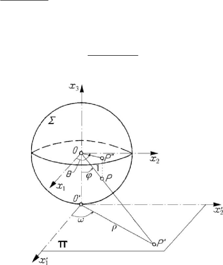
Figure 7.21. Transformation of a spherical motion.

lead to the motion of a particle

′

acted upon by a force which depends only on the

position (

()

′

′′

FFr) too; P. Appell showed that the trajectory of the particle P

′

the homographic transformation of the trajectory of the particle

P , the direction of the

force

′

F being also the homographic transformation of the direction of the force F . In

particular, if

F is a central force, then the force

′

F is a central one too or has a fixed

direction. One may also prove that the most general transformation of the form

()xx

αα

′′

r , 1, 2α = , d()dttλ

′

r , so that for any ()

FFr to have ()

′′′

=FFr,

is a homographic transformation.

MECHANICAL SYSTEMS, CLASSICAL MODELS

456

One may imagine also other transformations of interest, e.g., the transformation of a

spherical motion (on a sphere) in a plane motion. Let thus be a sphere

Σ of radius

equal to unity (for the sake of simplicity) and of centre

O , and a plane Π tangent to

the sphere at the point

′

(Fig.7.21). By a central transformation, used in the

geographic map technique, to a point

P of longitude θ and colatitude ϕ on the sphere

we make to correspond a point

′

, of polar co-ordinates ,ρω, at which the radius OP

pierces the plane

Π ; thus, to the straight lines of the plane correspond great circles of

the sphere and inversely. We notice that

tanρϕ

, ωθ

. If the particle P is of

mass equal to unity, then the corresponding equations of motion on the sphere read

(

)

sin ( , )

ddtt

ϕΘθϕ=

(

)

sin cos ( , )

ϕϕ Φθϕ−=

;

(7.2.27)

as well, the equations of motion of a particle

′

of mass equal to unity in the plane Π

are written in the form

(

)

(, )

ρρω−=

′

(

)

(, )

ddtt

ρΩρω=

′′

(7.2.27')

P. Appell showed that, in the case of a central transformation for which

dcosdttϕ

′

= , the equations (7.2.27) become (7.2.27'), where

cosR Φϕ= ,

cosΩΘ ϕ= . Obviously, the plane motion may be studied easier than the spherical

one.

2.2.4 Motion on synchronous curves and surfaces

Let be – in a fixed plane – a family of curves

{

}

C , which depend on a parameter

and pass through the fixed point

. Let us launch from

, at the initial moment

tt=

, with initial velocities of equal modulus

v , identical particles

, acted upon by

forces which derive from a given potential; the locus of the positions of the particles

at the same moment

is the curve

. The curves

{

}

Γ form a family of curves which

depend on the parameter

t and are called synchronous curves of the curves

{

}

C . If

the family of curves

{

}

C belongs to the three-dimensional space, then the locus of the

positions of the particles

P at the same moment t is a surface Σ ; the family of

surfaces

{

}

depends on the parameter t and forms the synchronous surfaces of the

curves

{

}

C .

Euler showed that, if

, the given force corresponding to a gravitational field,

the lines

{

}

C being straight lines in a vertical plane and passing through

, then the

synchronous curves

{

}

Γ are circles.

Let be the family of lines

{

}

C , called trajectories, which pass through the point O ,

and the family of lines

{

}

′

, called synodal lines, which pass through the same point.

One may prove that there exists an infinity of given conservative forces

F so that a

particle departing from

O with a given initial velocity, along one of the lines

{

}

Problems of dynamics of the particle

457

reaches a point

P in the same interval of time in which it would reach it along that

curve

{

}

′

which would pass through the same point. Obviously, the families of

curves

{

}

and

{

}

′

may invert their rôles. We mention that, if the synchronous lines

are orthogonal to the trajectories, in a plane motion, then the latter ones coincide with

the synodal lines, being brachistochrones for the considered forces. These problems

have been studied by Fouret, Saint-Germain and Vâlcovici.

2.3 Stability of equilibrium of a particle

In what follows, we make some considerations concerning the stability of

equilibrium of a free or constraint particle, completing thus the results in Chap. 4,

Subsec. 1.1.5; the results thus obtained will be then used for representations in the

phase plane.

2.3.1 Stability of equilibrium of a free particle

In Chap. 4, Subsec. 1.1.7, we have presented the Lagrange-Dirichlet theorem, which

states that a position

P of a free particle P , acted upon by a field of conservative

forces is a position of stable equilibrium if the simple potential

U has an isolated

maximum at that point. The demonstration which has been given has rather an intuitive

character; we will use the conservation theorem of mechanical energy for a rigorous

demonstration.

We notice that the potential

()U r is determined making abstraction of an additive

constant; choosing the point

P as origin O , we may take (0) 0U

. Let be a closed

convex surface

S which contains the point O (e.g., a sphere of centre O ), of arbitrary

small dimensions, so that in the interior and on the surface the function

()U r be

negative, vanishing only at

O . We may assume that there exists 0p > sufficiently

small so that to have

Up−>, hence

0UP

on the surface

. Let

be an

initial position of the particle

in the interior of the surface

, the corresponding

velocity being

v ; taking into account the conservation theorem of mechanical energy,

we may write

(

)

/2 /2mv U mv U=+ − ,

. We may determine the

position and the magnitude of the velocity at the initial moment by the condition

/2mv U p−<; to do this, it is sufficient – for instance – to take

/2 /2mv p< ,

/2Up−< . The first relation shows that

/vpmη

′

. As well, the function

being continuous and vanishing at the origin, it results that there exists

0η > so that

OP η< , corresponding

/2Up−< . Thus, if – in the interior of the surface S – we

give to the particle an initial position at a distance of

O less than η , with an initial

velocity less than

′

, then the conservation theorem of mechanical energy leads to the

inequality

/2mv U p<+, which proves that the particle cannot come out from the

interior of the surface

S ; indeed, if the particle P would reach the surface S , then the

sum

Up+ would become negative, situation impossible if we take into account the

previous relation. One may thus state that it corresponds an

0ε > , so that

OP ε<

MECHANICAL SYSTEMS, CLASSICAL MODELS

458

()PPt= . As well,

/2mv p

, because 0U

; it results () 2 /vt p m<

0ε

′

=>. The conditions that the point

≡

be a stable position of equilibrium are

thus fulfilled and the Lagrange-Dirichlet theorem is proved for a free particle. For

instance, for a free particle in rectilinear motion, acted upon by a force

()Fx kx=− ,

0k > , which derives from the simple potential

() /2Ux kx=− , the origin of the co-

ordinate axis represents a stable position of equilibrium.

This demonstration remains valid in the case of a generalized potential

U , where the

rôle of the function which has an isolated maximum is played by the scalar potential

U .

In what concerns the reciprocal of this theorem, the problem is not sufficiently

clarified. One may show that, in certain particular cases, a point may represent a stable

position of equilibrium, the potential

U having not an isolated maximum at that point.

Analogously, it is proved that a position of equilibrium

P is a position of labile

equilibrium if the potential

has an isolated minimum at that point. The conditions

imposed by the Lagrange-Dirichlet theorem are – obviously – sufficient conditions. A

more profound study of this problem will be made latter, after Lyapunov, in connection

with the study of the stability of motion in the frame of Lagrangian or Hamiltonian

mechanics. We mention the affirmation of T. Levi-Civita who said that “the instability

is the rule, while the stability is rather an exception”.

In the case of a non-conservative field of forces, the positions of equilibrium are

recognized – in general – using the property of definition, that is perturbing arbitrarily

such a position and studying the returning modality of the particle.

2.3.2 Stability of equilibrium of a particle subjected to constraints

In the case of a particle constrained to stay on a fixed smooth surface

S , one may

introduce the generalized forces

(,)Quv

, 1, 2α

, given by (4.1.47), as we have

seen in Chap. 4, Subsec. 1.1.7; if

ddd(,)Qu Qv Uuv+= , that is a total

differential, then we are led to the study of the extrema of the function

(,)UUuv= ,

where

u and v are generalized co-ordinates, the holonomic, scleronomic constraints

being eliminated. We may always make so as to have a maximum equal to zero for

U at the point

P coinciding with the origin ( (0,0) 0U

). We draw a closed curve

C around the point

, on the surface S , so that to have

on that curve;

hence, there exists

0p > so that 0Up

< on C . Displacing the particle from

at a neighbouring point, in the interior of the curve

C , we may follow the

demonstration given in the previous subsection, so that the Lagrange-Dirichlet

theorem is applicable in this case too.

Analogously, if the particle is constrained to stay on a fixed smooth curve

C , we

have seen in Chap. 4, Subsec. 1.1.7 too that the generalized force

()Qq , given by

(4.1.48) may be introduced, hence the function

() ()dUq Qq q=

∫

, being thus led to the

study of the isolated maxima of that function. We assume that

(0) 0U =

at the point

Problems of dynamics of the particle

459

P ; then we follow the previous demonstration, displacing the particle in the interior of

an arbitrary interval

[

]

,ηη− , which contains the point

P .

Using the potential energy

V given by (6.1.14), (6.1.14') and starting from the

Theorem 4.1.3, we may, finally, state

Theorem 7.2.2 (Lagrange-Dirichlet). The position of equilibrium

P of a particle P

subjected to holonomic, scleronomic constraints, in the presence of a field of

conservative forces, the potential energy having an isolated minimum at that point, is a

stable position of equilibrium.

This statement contains the case of the free particle as well the case of a constraint

one (in this case the potential energy must be expressed by means of generalized co-

ordinates, eliminating the constraint relations), where the conservative field may derive

from a simple or a generalized potential. If the potential energy has an isolated

maximum at the point

P , then that point represents a position of labile equilibrium.

In particular, in the case of a gravitational field

()Vmgx

r , one obtains the

Theorem 4.1.2 of Torricelli for a particle constrained to stay on a fixed smooth curve or

on a surface having the same properties.

2.3.3 Small oscillations of a heavy particle around the lowest point of a surface

Let be a surface

S which passes through the origin O , so that the tangent plane at

this point is horizontal, and the surface is over that plane in the vicinity of the respective

point. Corresponding to Torricelli’s theorem, the point

O is a stable position of

equilibrium for a heavy particle

P . Taking the

Ox -axis along the local ascendent

vertical, the surface

S may be represented in the neighbourhood of the point O by a

Maclaurin series of the form

312

(, )

xxx

⎛⎞

=++

⎜⎟

⎝⎠

(7.2.28)

where

R and

R are the principal radii of curvature (the extreme values of the radii

ρ ) of the surface at O , while

(, )xxϕ corresponds to terms of at least the third

degree with respect to the co-ordinates

,xx. Let us consider the small motions of the

particle

P around the point O . The simple potential which corresponds to the

gravitational field is

()Ux mgx

− ; eliminating the constraint relation (7.2.28) and

neglecting terms of higher order, we obtain

(, )

Ux x

⎛⎞

=− +

⎜⎟

⎝⎠

and the force which acts upon the particle is given by

grad

Umg

⎛⎞

==− +

⎜⎟

⎝⎠

Fii.

MECHANICAL SYSTEMS, CLASSICAL MODELS

460

We obtain thus the equations of motion

111

xxω=− ,

222

xxω=− ,

ω =

(7.2.29)

Integrating, it results

11 1 1

cos( )xa tωϕ=−,

22 2 2

cos( )xa tωϕ

− ,

(7.2.29')

where the amplitudes

,aa and the phase shifts

,ϕϕ are determined by the initial

conditions. In particular, if

RRR

, then one obtains the small motions

corresponding to the spherical pendulum (see Subsec. 1.3.7); the general case will be

studied in Chap. 8, Subsec. 2.2.5.

2.3.4 Representations in the phase plane. Topological methods

In Chap. 6, Subsec. 2.2.4 we have seen how one may study the motion of a particle

with a single degree of freedom in the conservative case of equation

()qfq= in the

phase space of co-ordinates

,qp; the results thus obtained may be applied for linear

systems as well as for non-linear ones. As an example, we consider the simple

pendulum (see Subsec. 1.3.1) for which (

q θ

)

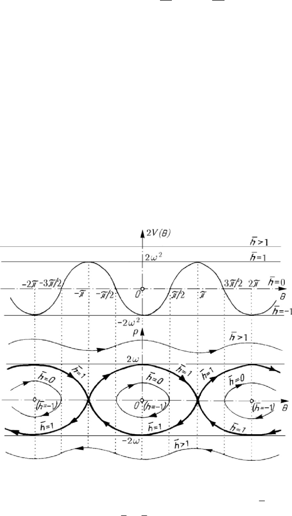
Figure 7.22. Simple pendulum; representation of the motion in the phase plane.

2cosphωθ=+, p θ



() cosV θωθ=− ,

2hhω

, cosh α

− ,