Sundararaja D. The Discrete Fourier Transform. Theory, Algorithms and Applications

Подождите немного. Документ загружается.

254

The Continuous-Time Fourier Series

x(0),x(£),x(2^),...,x((N-l)$). Then, Eq. (12.3) is approximated as

T *->

" N N

n=0 n=0

Since x(nT

) represents the nth sample, the equation can be rewritten as

JV_1

(k)

= -

£x(n)e-

i¥nk

, k =

0,l,...,N-l

71=0

This equation analyzes a waveform in terms of sinusoids. The inverse oper-

ation, that is the synthesis of a waveform from the coefficients, Eq. (12.2),

is approximated as

JV-l

x(n) = Y,

{k)e^

n =

0,l,...,N-l.

One difference between the DFT equation and the numerical approximation

to the FS is the factor jj. Therefore, by dividing the DFT coefficients by

N, we get an approximation to the complex FS coefficients. Comparing the

approximation of the synthesis equation with the IDFT equation, we find

that there is no constant divisor ^ in the synthesis equation. For N even,

comparing the coefficients of the DFT with that of the FS, we get, for real

signals,

(k)

= |pRe(X(fc)), X

(k) = -^Im(X(k)), k =

1,2,...,

y - 1

(k)

= ^-, * = 0,l,...,y-l and Re(X

(^)) = ^

Errors arise in DFT processing because of the digital representation of the

data and coefficients, and the round off of numbers in arithmetic operations,

as in any numerical computation using digital devices.

Aliasing effect

Once we represent the signal by N samples, we are able to compute only

N distinct frequency coefficients. If the input signal is bandlimited to

components with frequency indices less than ^i then there is no problem.

The 1-D Continuous-Time Fourier Series

255

Otherwise, the aliasing effect, described in terms of time-domain signals in

the last chapter, corrupts the spectrum. Consider the synthesis of a signal,

x(t) =

Xcs(iw

laot

l=—oo

where u>o =

%jr.

Let T

— ]j. To generate only samples of the signal at

intervals of T

, we get

oo oo

x(nT

) = J2

{l)e

iluonT

= £

.(I)e>*

l=—oo l=—oo

Let I = k + rN, where r = —oo,...,

—1,0,1,...,

oo. Then,

JV-1 oo N-l oo

(nT

) = Y, J2 Xcs(k+rN)e

k+rN

)

= Y, H

+ rN)e

k=0 r=—oo fc=0 r=—oo

We use X)^l-oo

+ rN) to get the samples of continuous-time signal

x(t).

Comparing this equation with that of the IDFT, we find that

X(k) = N ]T

+ rN), fc = 0,1,...,JV-l

r= —oo

This equation shows how the DFT coefficients are corrupted due to aliasing.

Example 12.1 The aliasing effect

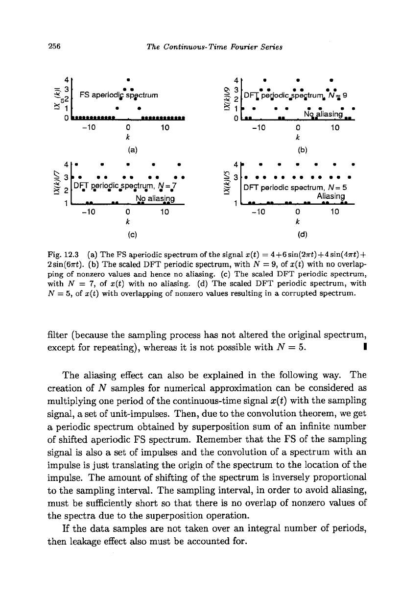
Figure 12.3(a) shows the FS magnitude spectrum, which is aperiodic, of

the signal x(t) =4 + 6 sin(27r£) + 4 sin 2(27ri) +

sin

3(27ri).

The signal has

frequency components, apart from dc, with frequencies 1 Hz, 2 Hz, and 3

Hz. Therefore, we need a minimum of seven samples in a period to represent

it accurately. Figure 12.3(b) shows the scaled DFT periodic spectrum which

is a superposition sum of the aperiodic spectrum placed at intervals of

nine samples. As the interval of nine samples is more than adequate to

prevent overlap of nonzero values of the spectrum, there is no aliasing effect.

Figure 12.3(c) shows the scaled DFT periodic spectrum with a period of

seven samples and there is no aliasing effect. Figure 12.3(d) shows the

scaled DFT periodic spectrum which is a corrupted periodic version of the

aperiodic spectrum. This is because the period of five samples is inadequate

to prevent the overlap of nonzero values of the aperiodic spectrum. The

magnitude of the spectral value with index 2 is one. We can recover the

original signal from its samples with N = 7 and N = 9 using a lowpass

256

The Continuous-Time Fourier Series

"B2

FS aperiodij spgctrum

S 2

* 1

• • • • • •

DFT,

pegodic^spejtrurr^ /V= 9

aliasing ..

-10

(a)

10 -10

(b)

& 2

DFT periodic spectrum, N = 7

No aliasinq

§.3

DFT periodic spectrum, N= 5

Aliasing

-10

(c)

-10

(d)

Fig. 12.3 (a) The FS aperiodic spectrum of the signal x(t) = 4 + 6sin(27rt)-f 4 sin(4n-t)+

2sin(67rt). (b) The scaled DFT periodic spectrum, with N = 9, of i(t) with no overlap-

ping of nonzero values and hence no aliasing, (c) The scaled DFT periodic spectrum,

with N = 7, of x(t) with no aliasing, (d) The scaled DFT periodic spectrum, with

N = 5, of x(t) with overlapping of nonzero values resulting in a corrupted spectrum.

filter (because the sampling process has not altered the original spectrum,

except for repeating), whereas it is not possible with N = 5. I

The aliasing effect can also be explained in the following way. The

creation of N samples for numerical approximation can be considered as

multiplying one period of the continuous-time signal x(t) with the sampling

signal, a set of unit-impulses. Then, due to the convolution theorem, we get

a periodic spectrum obtained by superposition sum of an infinite number

of shifted aperiodic FS spectrum. Remember that the FS of the sampling

signal is also a set of impulses and the convolution of a spectrum with an

impulse is just translating the origin of the spectrum to the location of the

impulse. The amount of shifting of the spectrum is inversely proportional

to the sampling interval. The sampling interval, in order to avoid aliasing,

must be sufficiently short so that there is no overlap of nonzero values of

the spectra due to the superposition operation.

If the data samples are not taken over an integral number of periods,

then leakage effect also must be accounted for.

The 1-D Continuous-Time Fourier Series 257

Continuous-time frequency

The DFT produces N output values corresponding to N input values and

the DFT computation is independent of the sampling interval T

. There-

fore,

the actual frequency can be found only if T

or T = NT

is known.

The fundamental frequency /o = ^ is also the frequency increment in Hz.

The DFT frequency index k represents a frequency of A;/

Hz. The DFT

time index n represents nT

seconds. The folding frequency is y/

and the

highest usable frequency is (y - l)/o.

Sample value at a discontinuity

At points of discontinuity of the function x(t), the average value

should be assigned to a sample, where x(t+) and x{t~) are the limiting

values of x(t) as t tends to t

from the right and left, respectively. In order

that the value x(t

) provides minimum least squares error,

(x(t

)-x(tt))

+ (x(t

)-x(t-))

must be minimum. Differentiating this expression with respect to x(t

) and

equating to zero, we get the result. In practice, it may be difficult to set the

sample value at each discontinuity to the average of the two immediately

adjacent values. This will introduce some error, which can be reduced by

increasing the number of samples.

Example 12.2 The approximation of the FS coefficients of a square

wave.

x(t) = |

A for 0 < t < £

0 for

< t < T

Solution

The waveform is odd-symmetric and odd half-wave symmetric with a dc

bias.

Therefore, we expect only the odd-indexed sine waves as the frequency

components, apart from the dc component.

1 /"= A

Xcs(0) = -J

Adt=-

258

The Continuous- Time Fourier Series

•5-

, Period, IT =1

•g.

0.5 '/v=4 >

Period T=1

0 2 4 6

(b)

io.;

• IMIMI

„ Period, r= 1

'W=16"

0 4 8 12

(c)

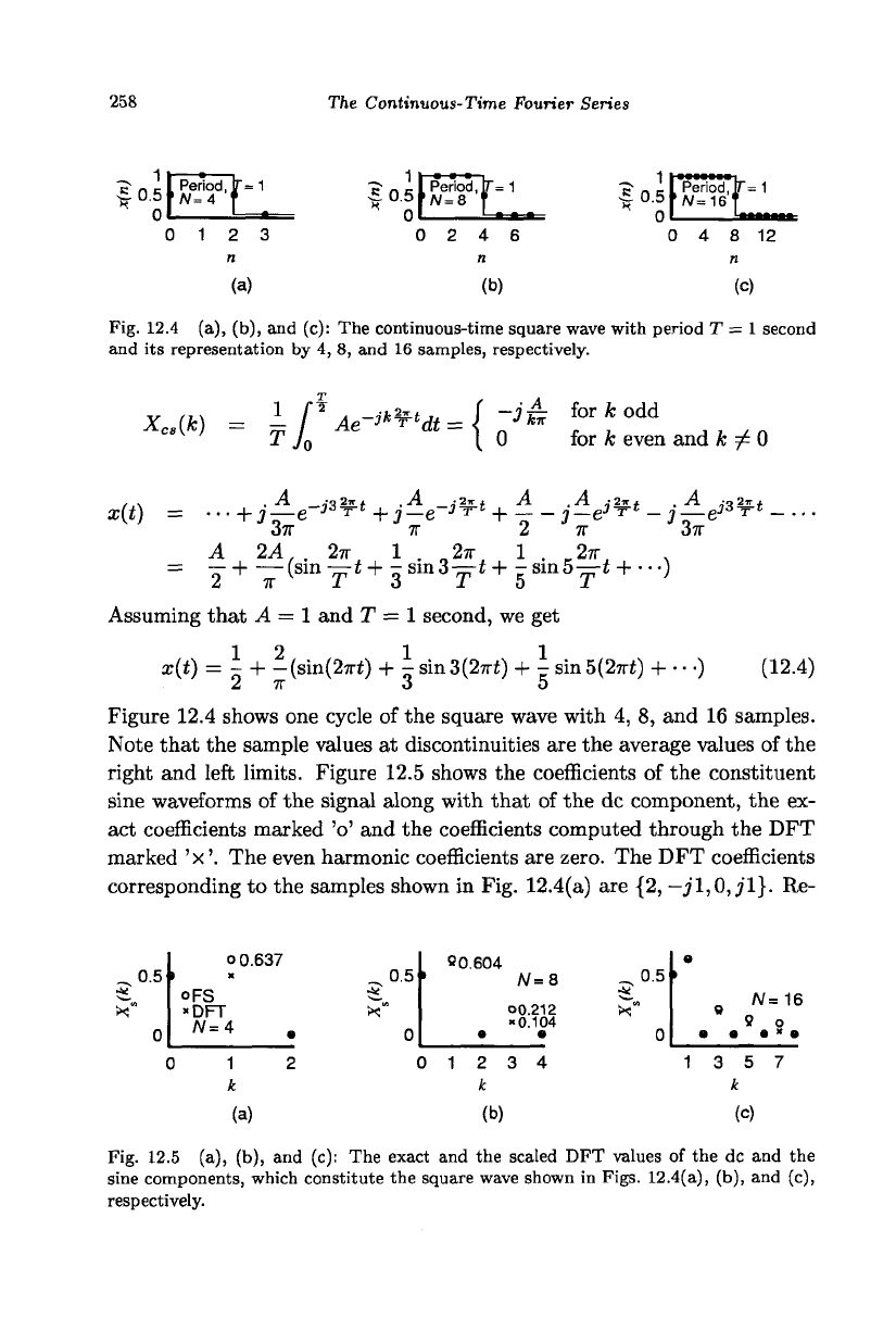
Fig. 12.4 (a), (b), and (c): The continuous-time square wave with period T = 1 second

and its representation by 4, 8, and 16 samples, respectively.

X (k) - - r Ae-f^dt-i ~

hrkodd

{k)

^ Ae

Q iolk ever

even and k ^0

37T

7T 2

24,

. 2?r 1 . 2TT 1 . 2TT

+ —(sin— i+-sm3—i+-sin5—< + •••)

x(t) = hj—e

~ 2

lSm

r' ' 3"~T' ' 5"""T

Assuming that A = 1 and T = 1 second, we get

V ' -|- " j — g^ V

j g^ T *

A „-2*

—<

12 1 1

a:(t) = - + -(sin(27rt) + - sin3(27rf) + - sin5(27ri) +

• •

•) (12.4)

2 7r 3 5

Figure 12.4 shows one cycle of the square wave with 4, 8, and 16 samples.

Note that the sample values at discontinuities are the average values of the

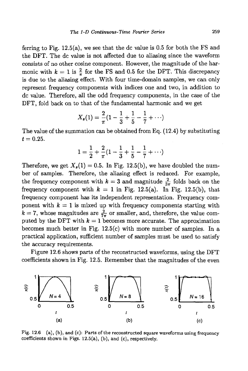
right and left limits. Figure 12.5 shows the coefficients of the constituent

sine waveforms of the signal along with that of the dc component, the ex-

act coefficients marked 'o' and the coefficients computed through the DFT

marked 'x'. The even harmonic coefficients are zero. The DFT coefficients

corresponding to the samples shown in Fig. 12.4(a) are {2, —

j'1,0,,7'1}.

Re-

0.5

0 0.637

oFS

»DFT

A/=4

0.5

00.604

W=8

00.212

»0.104

0 1

(b)

3 4

0.5

„ A/=16

° 9 o

• • • " •

13 5 7

(c)

Fig. 12.5 (a), (b), and (c): The exact and the scaled DFT values of the dc and the

sine components, which constitute the square wave shown in Figs. 12.4(a), (b), and (c),

respectively.

The 1-D Continuous-Time. Fourier Series 259

ferring to Fig. 12.5(a), we see that the dc value is 0.5 for both the FS and

the DFT. The dc value is not affected due to aliasing since the waveform

consists of no other cosine component. However, the magnitude of the har-

monic with k = 1 is \ for the FS and 0.5 for the DFT. This discrepancy

is due to the aliasing effect. With four time-domain samples, we can only

represent frequency components with indices one and two, in addition to

dc value. Therefore, all the odd frequency components, in the case of the

DFT, fold back on to that of the fundamental harmonic and we get

The value of the summation can be obtained from Eq. (12.4) by substituting

t = 0.25.

-, 1 2„ 1 1 1

^-a

s-^-)

Therefore, we get X

(l) = 0.5. In Fig. 12.5(b), we have doubled the num-

ber of samples. Therefore, the aliasing effect is reduced. For example,

the frequency component with k = 3 and magnitude ^ folds back on the

frequency component with k = 1 in Fig. 12.5(a). In Fig. 12.5(b), that

frequency component has its independent representation. Frequency com-

ponent with ifc = 1 is mixed up with frequency components starting with

k = 7, whose magnitudes are ^ or smaller, and, therefore, the value com-

puted by the DFT with k = 1 becomes more accurate. The approximation

becomes much better in Fig. 12.5(c) with more number of samples. In a

practical application, sufficient number of samples must be used to satisfy

the accuracy requirements.

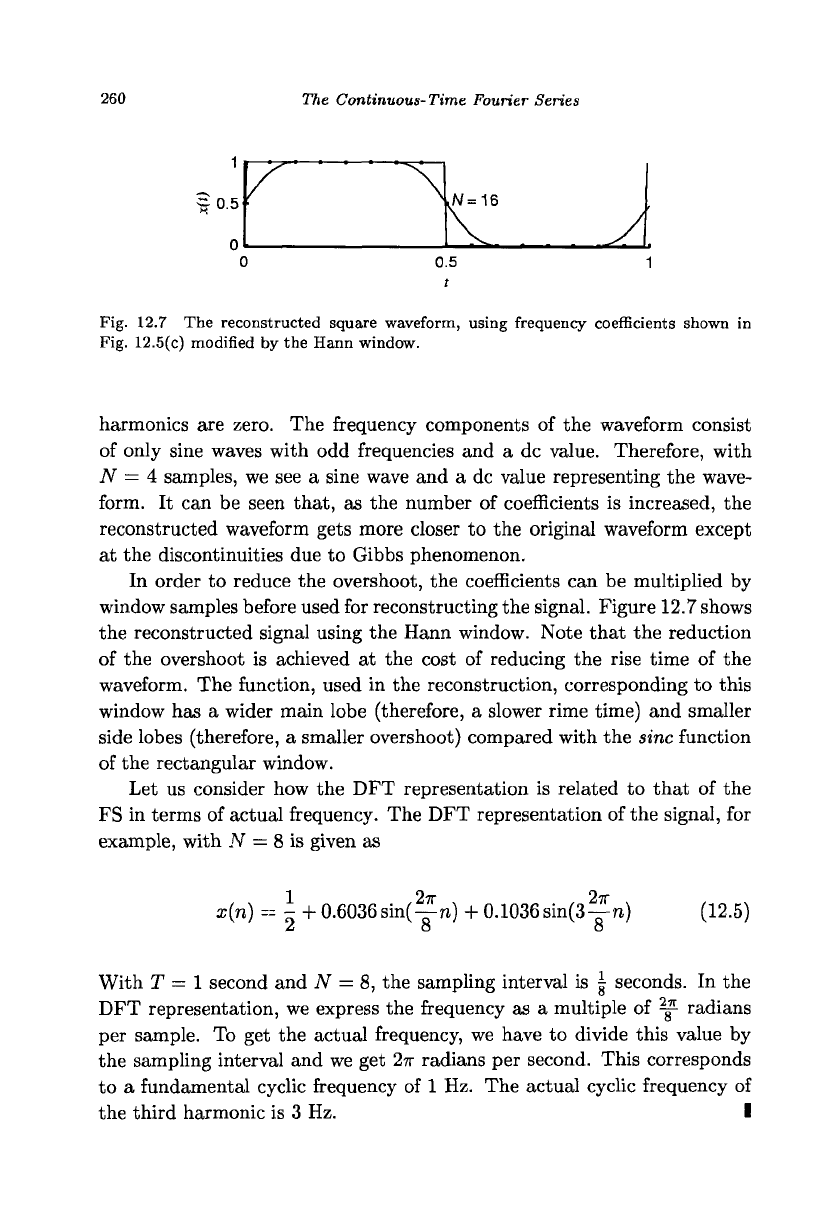
Figure 12.6 shows parts of the reconstructed waveforms, using the DFT

coefficients shown in Fig. 12.5. Remember that the magnitudes of the even

=* \

N=a

f "-is

0 0.5 0 0.5 0 0.5

i t t

(a) (b) (c)

Fig. 12.6 (a), (b), and (c): Parts of the reconstructed square waveforms using frequency

coefficients shown in Figs. 12.5(a), (b), and (c), respectively.

260 The Continuous- Time Fourier Series

S0.5

0 0.5 1

Fig. 12.7 The reconstructed square waveform, using frequency coefficients shown in

Fig. 12.5(c) modified by the Hann window.

harmonics are zero. The frequency components of the waveform consist

of only sine waves with odd frequencies and a dc value. Therefore, with

TV = 4 samples, we see a sine wave and a dc value representing the wave-

form. It can be seen that, as the number of coefficients is increased, the

reconstructed waveform gets more closer to the original waveform except

at the discontinuities due to Gibbs phenomenon.

In order to reduce the overshoot, the coefficients can be multiplied by

window samples before used for reconstructing the signal. Figure 12.7 shows

the reconstructed signal using the Hann window. Note that the reduction

of the overshoot is achieved at the cost of reducing the rise time of the

waveform. The function, used in the reconstruction, corresponding to this

window has a wider main lobe (therefore, a slower rime time) and smaller

side lobes (therefore, a smaller overshoot) compared with the sine function

of the rectangular window.

Let us consider how the DFT representation is related to that of the

FS in terms of actual frequency. The DFT representation of the signal, for

example, with N = 8 is given as

2TT 2TT

x(n) = -+ 0.6036 sin(-n) + 0.1036 sin(3—n) (12.5)

2 8 8

With T = 1 second and N = 8, the sampling interval is | seconds. In the

DFT representation, we express the frequency as a multiple of ^ radians

per sample. To get the actual frequency, we have to divide this value by

the sampling interval and we get

2TT

radians per second. This corresponds

to a fundamental cyclic frequency of 1 Hz. The actual cyclic frequency of

the third harmonic is 3 Hz. I

The 1-D Continuous-Time Fourier Series

261

1.1002

0.5

1.0901

0.5

LH = 13

0 0.0753 0.1907 0 0.0382 0.0969

0 0.0192 0.0486

(b)

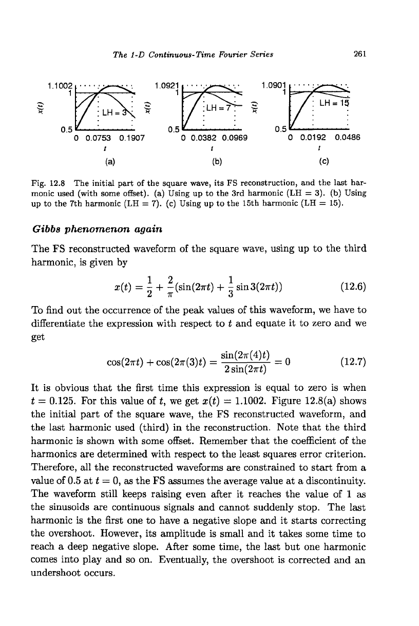
Fig. 12.8 The initial part of the square wave, its FS reconstruction, and the last har-

monic used (with some offset), (a) Using up to the 3rd harmonic (LH = 3). (b) Using

up to the 7th harmonic (LH = 7). (c) Using up to the 15th harmonic (LH = 15).

Gibbs phenomenon again

The FS reconstructed waveform of the square wave, using up to the third

harmonic, is given by

12 1

x(t) = - + -(sin(27rf) + - sin3(27ri))

7T 3

(12.6)

To find out the occurrence of the peak values of this waveform, we have to

differentiate the expression with respect to t and equate it to zero and we

get

cos(2

7ri

)+cos(2

r(3)i) = ^glM

0 (12.7)

It is obvious that the first time this expression is equal to zero is when

t = 0.125. For this value of t, we get x(t) =

1.1002.

Figure 12.8(a) shows

the initial part of the square wave, the FS reconstructed waveform, and

the last harmonic used (third) in the reconstruction. Note that the third

harmonic is shown with some offset. Remember that the coefficient of the

harmonics are determined with respect to the least squares error criterion.

Therefore, all the reconstructed waveforms are constrained to start from a

value of 0.5 at t = 0, as the FS assumes the average value at a discontinuity.

The waveform still keeps raising even after it reaches the value of 1 as

the sinusoids are continuous signals and cannot suddenly stop. The last

harmonic is the first one to have a negative slope and it starts correcting

the overshoot. However, its amplitude is small and it takes some time to

reach a deep negative slope. After some time, the last but one harmonic

comes into play and so on. Eventually, the overshoot is corrected and an

undershoot occurs.

262

The Continuous-Time Fourier Series

Figures 12.8(b) and (c) show the initial part of the square wave, the FS

reconstructed waveform, and the last harmonic used in the reconstruction,

the last harmonic being 7 and 15, respectively. We can easily calculate, as

shown earlier, that the first peak value occurs for these cases at t = 0.0625

and t = 0.03125, respectively. That is, the value of t for the occurrence

of the first peak value is reduced by a factor of 2 with the doubling of the

number of harmonics used for the reconstruction. The overshoot is also cor-

rected faster by a factor of

two.

With an infinite number of harmonics used,

the overshoot occurs almost at t = 0 and it exists only for a moment. The

largest overshoot converges to the value of

1.0895

with a relatively small

number of harmonics used. While the overshoot converges to a limit, the

area under the overshoot is reduced and eventually becomes zero confirm-

ing that the FS provides a complete representation for any waveform with

respect to the least squares error criterion. It should be noted that the FS

representation provides uniform convergence when the original waveform is

continuous. It is obvious because when the waveform is continuous the size

of discontinuity between adjacent points is zero and the overshoot=size of

discontinuity x 0.0895=0.

12.2 The 2-D Continuous-Time Fourier Series

The 2-D FS is a straightforward extension of the 1-D FS. A periodic signal,

x(ti, t

), satisfying the Dirichlet conditions, with periods T\ and T

, can be

equivalently expressed as

00 00

x(h,t

) = Y, E X

(kx,k

jmkltl

juJ2k2t

where wi = §£ and

= §£, and

.(*i,fe) = =V f ' f

x{t

)e-^

^e-^

^dt

J1J2 Jo Jo

Example 12.3 Find the 2-D FS of the continuous-time signal, a period

of which is defined as

2ir

x{h,t

) = sin(—ti), 0 < h < 3, 0 < t

< 2

Compute the 2-D DFT of the signal with 4 samples in each direction.

The 2-D Continuous-Time Fourier Series

263

Solution

. ,, 27r 2TT .

X{tl,t

) = Bin(lyti+Oyta)

j2^

;

^e.(l,0) = -|, X

(-l,0) = |

It is instructive to derive the FS coefficients directly from the definition.

The frequency components in the h direction is analyzed as

(kut2)

sin

(y*i)

e_j(¥fclil)di

Let wi = ?f. Then,

\ g—jkiuiti

{k±,t

)

= 3 /-. _

(~J

i"i

sin(o;iti) - ui cos(aJiti))|jj

= 0, fa ^ ±1

The numerator and the denominator evaluate to zero for fa = ±1. There-

fore,

we apply l'hopital's rule by differentiating the numerator and the

denominator separately with respect to fa and evaluate the limit to get

(±l,t

)

= T^

The frequency components in the t

direction is analyzed as

(^7>

J\^_ |2

i' -J7Tk

'°

= 0, k

# 0

The numerator and the denominator evaluate to zero for k

= 0. Therefore,

we apply l'hopital's rule and evaluate the limit to get

X„(±1,0) = ^