Sundararaja D. The Discrete Fourier Transform. Theory, Algorithms and Applications

Подождите немного. Документ загружается.

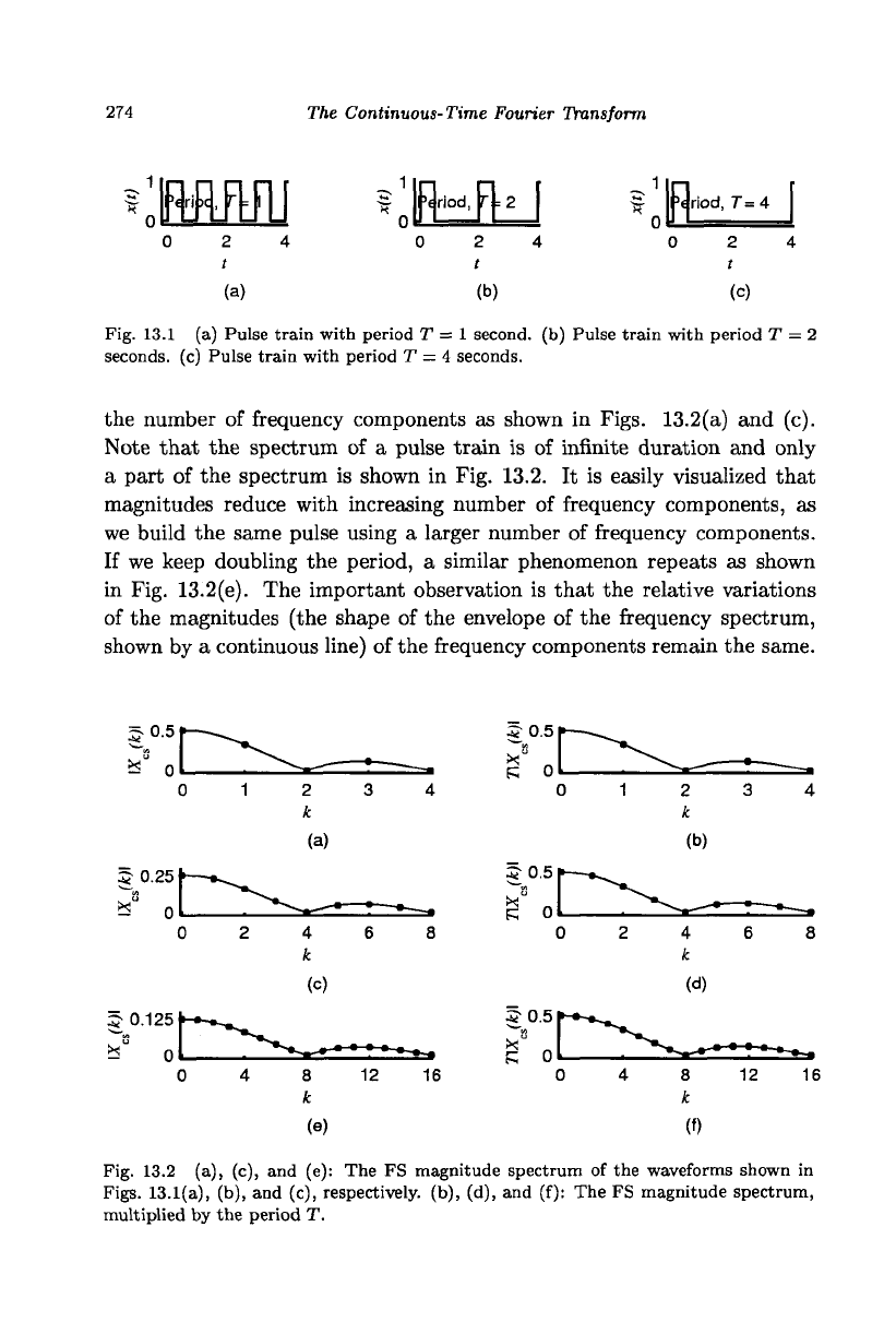
274

The Continuous-Time Fourier Transform

KMM1 ?Md Kft

iriod,

T= 4

(a)

(b) (c)

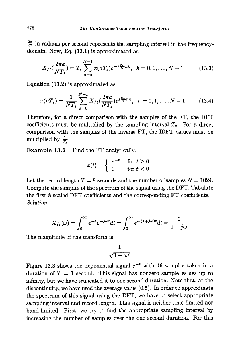
Fig. 13.1 (a) Pulse train with period T = 1 second, (b) Pulse train with period T = 2

seconds, (c) Pulse train with period T

—

4 seconds.

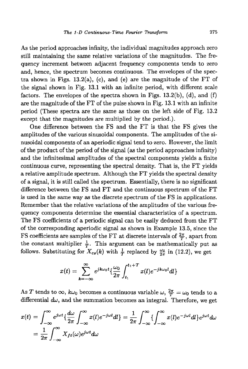
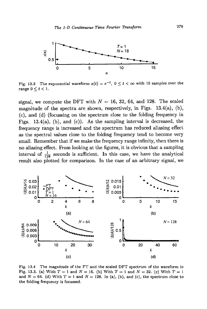
the number of frequency components as shown in Figs. 13.2(a) and (c).

Note that the spectrum of a pulse train is of infinite duration and only

a part of the spectrum is shown in Fig. 13.2. It is easily visualized that

magnitudes reduce with increasing number of frequency components, as

we build the same pulse using a larger number of frequency components.

If we keep doubling the period, a similar phenomenon repeats as shown

in Fig. 13.2(e). The important observation is that the relative variations

of the magnitudes (the shape of the envelope of the frequency spectrum,

shown by a continuous line) of the frequency components remain the same.

(a)

(c)

(e)

(b)

(d)

Fig. 13.2 (a), (c), and (e): The FS magnitude spectrum of the waveforms shown in

Figs.

13.1(a), (b), and (c), respectively, (b), (d), and (f): The FS magnitude spectrum,

multiplied by the period T.

The 1-D

Continuous-Time Fourier Transform

275

As the period approaches infinity, the individual magnitudes approach zero

still maintaining the same relative variations of the magnitudes. The fre-

quency increment between adjacent frequency components tends to zero

and, hence, the spectrum becomes continuous. The envelopes of the spec-

tra shown in Figs. 13.2(a), (c), and (e) are the magnitude of the FT of

the signal shown in Fig. 13.1 with an infinite period, with different scale

factors. The envelopes of the spectra shown in Figs. 13.2(b), (d), and (f)

are the magnitude of the FT of the pulse shown in Fig. 13.1 with an infinite

period (These spectra are the same as those on the left side of Fig. 13.2

except that the magnitudes are multiplied by the period.).

One difference between the FS and the FT is that the FS gives the

amplitudes of the various sinusoidal components. The amplitudes of the si-

nusoidal components of an aperiodic signal tend to zero. However, the limit

of the product of the period of the signal (as the period approaches infinity)

and the infinitesimal amplitudes of the spectral components yields a finite

continuous curve, representing the spectral density. That is, the FT yields

a relative amplitude spectrum. Although the FT yields the spectral density

of a signal, it is still called the spectrum. Essentially, there is no significant

difference between the FS and FT and the continuous spectrum of the FT

is used in the same way as the discrete spectrum of the FS in applications.

Remember that the relative variations of the amplitudes of the various fre-

quency components determine the essential characteristics of a spectrum.

The FS coefficients of a periodic signal can be easily deduced from the FT

of the corresponding aperiodic signal as shown in Example 13.5, since the

FS coefficients are samples of the FT at discrete intervals of ^, apart from

the constant multiplier y. This argument can be mathematically put as

follows. Substituting for

(k)

with ^ replaced by |£ in (12.2), we get

°° u

ti+T

;(t) = Y

J^ot{ o /

(l)e-

jkuol

dl}

™

Jti

As T tends to oo,

kuiQ

becomes a continuous variable

LJ,

^ = wo tends to a

differential dw, and the summation becomes an integral. Therefore, we get

^{ir- / x{l)e-

iu,

dl] = £- / { / x(l)e-

jul

dl}e

jut

cLj

-oo

i7r

J-oo to J-oo J-oo

i r°°

276

The Continuous-Time Fourier Transform

Therefore, the FT of the signal x(t) is defined as

x(t)e-

jut

dt (13.1)

-oo

The inverse FT of the transform Xf

(u) is defined as

1 r°°

x(t) = — / Xf

(u)e?

dw (13.2)

The sufficient conditions for the existence of FT are essentially the same as

those for the FS. Gibbs phenomenon is also common to both the FS and

the FT.

Example 13.1 Find the FT of the unit impulse signal x(i)

—

5{i).

8{t)e-

jult

dt = 1 and 5{t) & 1

•oo

That is, the unit impulse signal is composed of complex sinusoids of all

frequencies from u — — oo to a; = oo in equal proportion. I

Example 13.2 Find the inverse FT of the transform Xf

(uj) = 8(UJ).

1 f°° 1

x(t) = — 6(oj)e

jut

dui = — and 1 O 2ir6(u)

2-K J_

That is, the dc signal has nonzero spectral component only at u = 0. I

Example 13.3 Find the FT of the signal x{t) = eP

Uot

This signal can be considered as the product of signals x{t) = 1 and x(t) =

jwot Therefore, using the shift theorem e^

x(t)

<S>

Xft(u)—w

) and from

the result of Example 13.2, we get

iuot

«• 2-K6(UJ - u>

)

That is, the spectrum of the complex sinusoid with u =

u>o

is a single

impulse at u

—

UIQ.

Example 13.4 Find the FT of the signal x(t) =

COS(CJO^)-

OO I /-OO

cos{u

t)e-

jut

dt =- (e^

+ e-

juJot

)e-i

-OO

2 ./-oo

— Tr(6(u! -

UIQ)

+ 6(iJ + W

))

The 1-D Continuous-Time Fourier Transform

277

Hence, cos(ui

t) O ir(5(u - ui

) + S(u +

))-

Similarly, sin(u;o*) 4* {-j)ir(6(u ~

o) -

&(w

+ wo))-

Example 13.5 Find the FT of the signal x(t) =

From the Xf

(u) obtained, deduce the complex FS coefficients

(k)

if one

period of a periodic signal is defined as

{

1 0<t<a

0 a<t<T-a

1 T-a<t<T

where T = 5 seconds and a = | seconds.

Solution

As the signal is even-symmetric,

(u)

= 2 / cos(wi) dt = 2—^—-

Since X

(fc) = ^Xf

(kuJo), with a = |, T = 5, and w

get

^.« = I

^ = ^,M0 and

The relation between the DFT and the FT

Comparing with the approximation of the FS by the DFT, the difference in

the approximation of the samples of the FT is that we truncate the signal,

which could be of infinite length, to a finite length T. Now, the signal is

assumed periodic of period T. The consequence of truncation is that the

spectrum is distorted, since the resulting spectrum is the convolution of the

spectra of the given signal and the rectangular window. But for truncation,

the approximation of the samples of the FT by the DFT is the same as that

of the FS.

Let us approximate the integral in Eq. (13.1) using the rectangular

rule of numerical integration. The summation interval can start from zero,

since we assume periodicity, although the input signal can be nonzero in

any interval. We divide the period T into N intervals of width T

= jj and

represent the signal at N points as x(0),x(^-),x(2^),.. .,x((N-l)^). T

in seconds represents the sampling interval in the time-domain and -r£r =

J 1 for

—

a <t < a

1 0 elsewhere

koj

= k~, we

*»(0) =

278

The Continuous-Time Fourier Transform

Y~ in radians per second represents the sampling interval in the frequency-

domain. Now, Eq. (13.1) is approximated as

*•

(-£

= T.Y

<nT

)e-i

B-

0,1,..

.,N -

1 (13.3)

n=0

Equation (13.2)

approximated as

<nTs)

WF ^

Mj£fy

¥nk

> n

0,l,...,N-l

(13.4)

fc=o

Therefore,

for a

direct comparison with the samples

the FT, the DFT

coefficients must

multiplied by the sampling interval

For

direct

comparison with the samples of the inverse FT, the IDFT values must

multiplied by

£-.

Example 13.6 Find the FT analytically.

, fe"'

for

t > 0

x(t)

0 for *

< 0

Let the record length

—

8 seconds and the number of samples

N =

1024.

Compute the samples of the spectrum of the signal using the DFT. Tabulate

the first

scaled DFT coefficients and the corresponding FT coefficients.

Solution

/•OO

y-OO -I

(w)=

e-*e->

dt= e^

1+ju)t

dt=

1 +

JUJ

The magnitude of the transform

N/TT

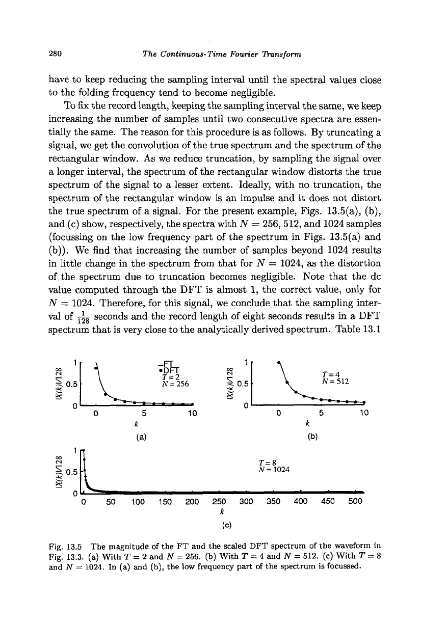
Figure 13.3 shows the exponential signal

-t

with 16 samples taken

in a

duration

of T = 1

second. This signal has nonzero sample values

up to

infinity, but we have truncated

to one second duration. Note that, at the

discontinuity, we have used the average value (0.5). In order to approximate

the spectrum of this signal using the DFT, we have to select appropriate

sampling interval and record length. This signal is neither time-limited nor

band-limited. First, we try

find the appropriate sampling interval

increasing the number

samples over the one second duration. For this

The 1-D Continuous-Time Fourier Transform

279

Fig. 13.3 The exponential waveform x(t) = e

, 0 < t < oo with 16 samples over the

range 0 < t < 1.

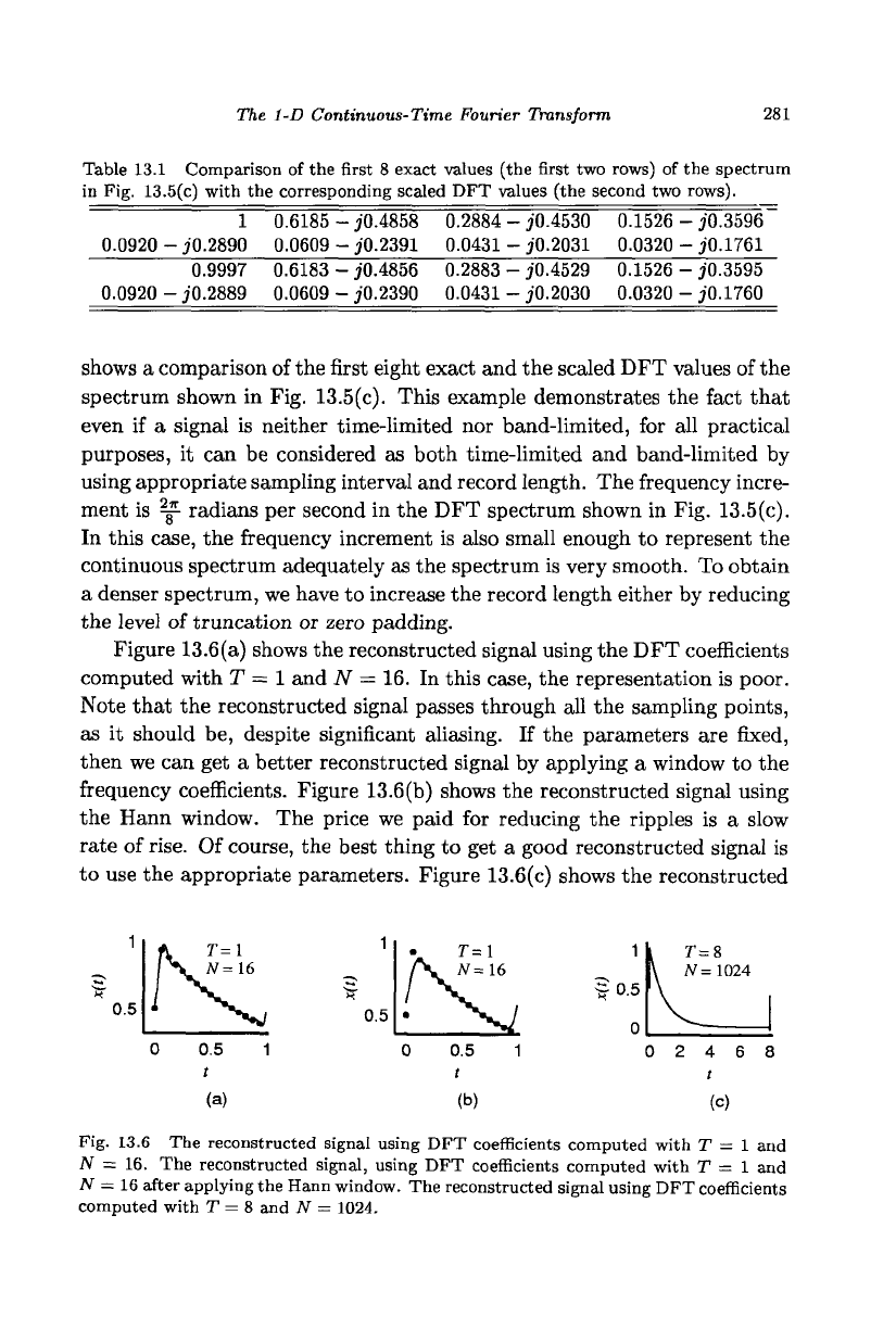
signal, we compute the DFT with N = 16, 32, 64, and 128. The scaled

magnitude of the spectra are shown, respectively, in Figs. 13.4(a), (b),

(c),

and (d) (focussing on the spectrum close to the folding frequency in

Figs.

13.4(a), (b), and (c)). As the sampling interval is decreased, the

frequency range is increased and the spectrum has reduced aliasing effect

as the spectral values close to the folding frequency tend to become very

small. Remember that if we make the frequency range infinity, then there is

no aliasing effect. From looking at the figures, it is obvious that a sampling

interval of j^g seconds is sufficient. In this case, we have the analytical

result also plotted for comparison. In the case of an arbitrary signal, we

*2 0.03

5 0.02

&0.01

-FT

•DFT

T=\

W=16

3 0.009

0.006

& 0.003

10 20

(c)

2 0.015

5; 0.01

S" 0.005

.0.5

/V = 32

5 10 15

(b)

W=128

20 40 60

(d)

Fig. 13.4 The magnitude of the FT and the scaled DFT spectrum of the waveform in

Fig. 13.3. (a) With T = 1 and N = 16. (b) With T = 1 and N = 32. (c) With T = 1

and N = 64. (d) With T = 1 and N = 128. In (a), (b), and (c), the spectrum close to

the folding frequency is focussed.

280

The Continuous-Time Fourier Transform

have to keep reducing the sampling interval until the spectral values close

to the folding frequency tend to become negligible.

To fix the record length, keeping the sampling interval the same, we keep

increasing the number of samples until two consecutive spectra are essen-

tially the same. The reason for this procedure is as follows. By truncating a

signal, we get the convolution of the true spectrum and the spectrum of the

rectangular window. As we reduce truncation, by sampling the signal over

a longer interval, the spectrum of the rectangular window distorts the true

spectrum of the signal to a lesser extent. Ideally, with no truncation, the

spectrum of the rectangular window is an impulse and it does not distort

the true spectrum of a signal. For the present example, Figs. 13.5(a), (b),

and (c) show, respectively, the spectra with N = 256, 512, and 1024 samples

(focussing on the low frequency part of the spectrum in Figs. 13.5(a) and

(b)).

We find that increasing the number of samples beyond 1024 results

in little change in the spectrum from that for N = 1024, as the distortion

of the spectrum due to truncation becomes negligible. Note that the dc

value computed through the DFT is almost 1, the correct value, only for

N = 1024. Therefore, for this signal, we conclude that the sampling inter-

val of j-|g seconds and the record length of eight seconds results in a DFT

spectrum that is very close to the analytically derived spectrum. Table 13.1

0.5

-FT

•DFT

T=2

N=256

0.5

T = 4

512

.0.5

r=8

N = 1024

(b)

100 150 200

250

300 350 400 450 500

(c)

Fig. 13.5 The magnitude of the FT and the scaled DFT spectrum of the waveform in

Fig. 13.3. (a) With T = 2 and N - 256. (b) With T = 4 and TV = 512. (c) With T = 8

and N = 1024. In (a) and (b), the low frequency part of the spectrum is focussed.

The 1-D Continuous-Time Fourier Transform

281

Table 13.1 Comparison of the first 8 exact values (the first two rows) of the spectrum

in Fig. 13.5(c) with the corresponding scaled DFT values (the second two rows).

0.0920 - jO.2890

0.6185-J0.4858

0.0609 - jO.2391

0.2884 - jO.4530

0.0431 - jO.2031

0.1526-jO.3596"

0.0320 -jO.1761

0.9997 0.6183 - jO.4856 0.2883-jO.4529 0.1526 - jO.3595

0.0920 - jO.2889 0.0609 - jO.2390 0.0431 - jO.2030 0.0320 - j'0.1760

shows a comparison of the first eight exact and the scaled DFT values of the

spectrum shown in Fig. 13.5(c). This example demonstrates the fact that

even if a signal is neither time-limited nor band-limited, for all practical

purposes, it can be considered as both time-limited and band-limited by

using appropriate sampling interval and record length. The frequency incre-

ment is ^2- radians per second in the DFT spectrum shown in Fig. 13.5(c).

In this case, the frequency increment is also small enough to represent the

continuous spectrum adequately as the spectrum is very smooth. To obtain

a denser spectrum, we have to increase the record length either by reducing

the level of truncation or zero padding.

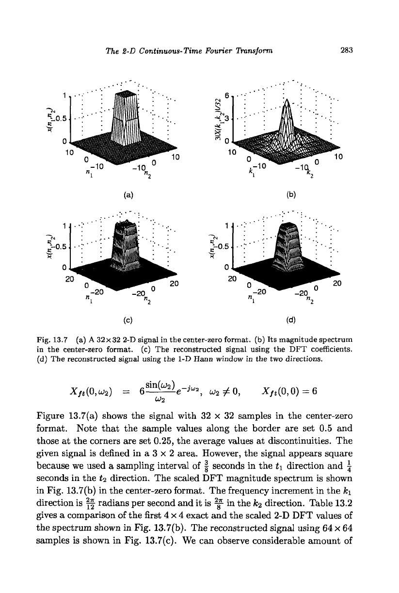
Figure 13.6(a) shows the reconstructed signal using the DFT coefficients

computed with T = 1 and N = 16. In this case, the representation is poor.

Note that the reconstructed signal passes through all the sampling points,

as it should be, despite significant aliasing. If the parameters are fixed,

then we can get a better reconstructed signal by applying a window to the

frequency coefficients. Figure 13.6(b) shows the reconstructed signal using

the Hann window. The price we paid for reducing the ripples is a slow

rate of rise. Of course, the best thing to get a good reconstructed signal is

to use the appropriate parameters. Figure 13.6(c) shows the reconstructed

0.5

T=\

N=16

0.5

(a)

(b)

0 2 4 6 8

(c)

Fig. 13.6 The reconstructed signal using DFT coefficients computed with T = 1 and

N = 16. The reconstructed signal, using DFT coefficients computed with T = 1 and

N = 16 after applying the Hann window. The reconstructed signal using DFT coefficients

computed with T = 8 and N = 1024.

282

The Continuous-Time Fourier Transform

signal using DFT coefficients computed with T = 8 and N = 1024, which

is quite close to the original signal (Notice the overshoot and undershoot

at the discontinuity due to Gibbs phenomenon.). I

In summary, a trial and error procedure is used to approximate the

spectrum of an arbitrary signal by the DFT. First, select the appropriate

sampling interval. This is done by selecting a reasonable record length

and trying with different sampling intervals so that spectral values close

to the folding frequency are sufficiently small. The second step is to keep

the sampling interval the same and try different record lengths. The record

length is chosen so that changes in the spectrum with a longer record length

is negligible.

13.2 The 2-D Continuous-Time Fourier Transform

The 2-D FT is a straightforward extension of the 1-D FT.

oo roo

/ x(t

)e-

ltl

*dt

-oo J—oo

-I rOO /"OO

x(ti,t

) =

/ ^(wi.waJe^V^dwidwa

^™ J—oo J—oo

Example 13.7 Find the 2-D FT analytically.

u ^ _ J - for 0 < ii < 3, 0 < i

< 2

*(*i.'

)-<{ n

here

Let the record length Ti = 12 and T

= 8 seconds and the number of sam-

ples

Ni,N

= 32. Compute the samples of the spectrum of the signal using

the DFT. Tabulate the first 4x4 scaled DFT coefficients and the corre-

sponding FT coefficients. Reconstruct the signal using the DFT coefficients

with and without applying the Hann window.

Solution

As the signal is separable, we use the 1-D FT results to get

i \ sin(1.5wi)sin(w

) _,-a

_,-

(u!i,u

)

= 4—i '-—^—-e

JW2

, wi, ui

U)\

The 2-D Continuous-Time Fourier Transform

283

(a)

(b)

,-0.5

Z-0.5

(c)

(d)

Fig. 13.7 (a) A

2-D signal in the center-zero format, (b) Its magnitude spectrum

in the center-zero format, (c) The reconstructed signal using the DFT coefficients.

(d) The reconstructed signal using the 1-D Hann window in the two directions.

(0,uj

)

= 6^)e-'-, a* # 0,

(0,0) = 6

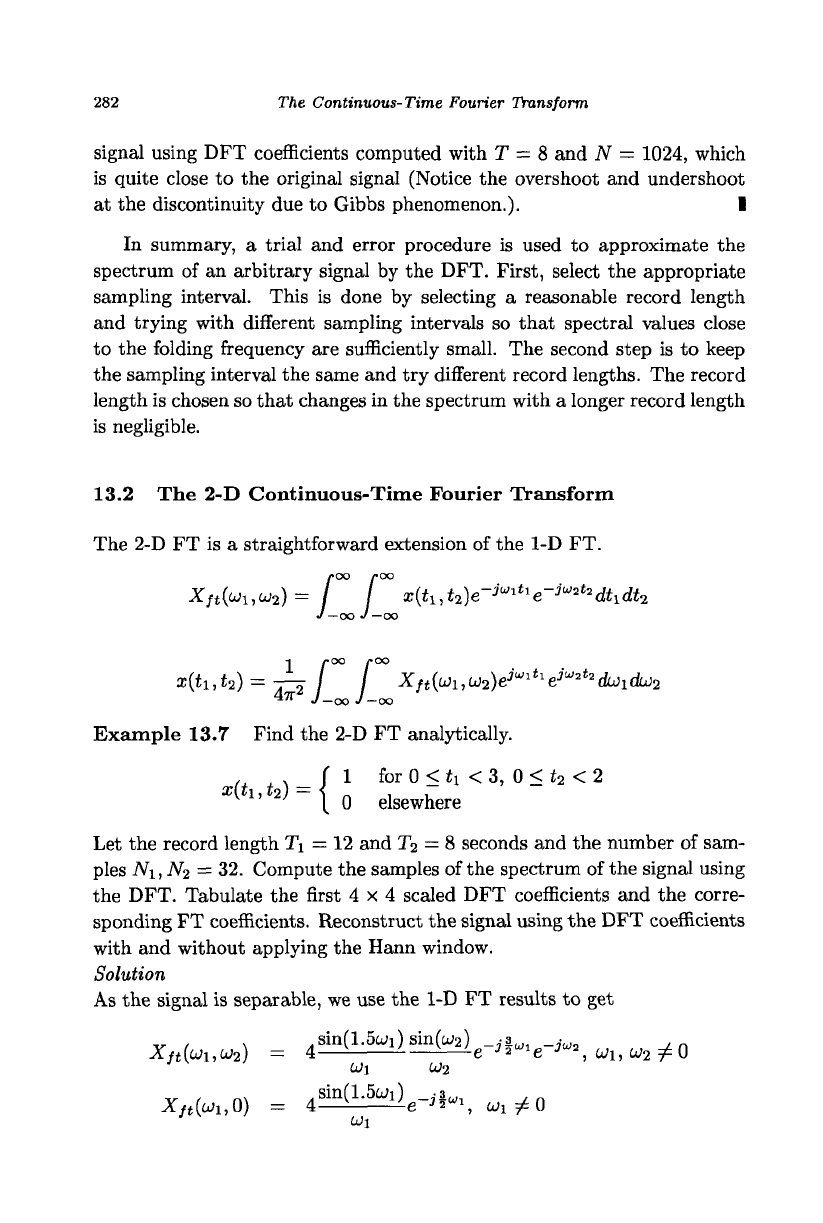
Figure 13.7(a) shows the signal with 32 x 32 samples in the center-zero

format. Note that the sample values along the border are set 0.5 and

those at the corners are set 0.25, the average values at discontinuities. The

given signal is defined in a 3 x 2 area. However, the signal appears square

because we used a sampling interval of | seconds in the t\ direction and \

seconds in the £

direction. The scaled DFT magnitude spectrum is shown

in Fig. 13.7(b) in the center-zero format. The frequency increment in the fci

direction is ff radians per second and it is ^ in the fc

direction. Table 13.2

gives a comparison of the first 4x4 exact and the scaled 2-D DFT values of

the spectrum shown in Fig. 13.7(b). The reconstructed signal using 64 x 64

samples is shown in Fig. 13.7(c). We can observe considerable amount of