Sundararaja D. The Discrete Fourier Transform. Theory, Algorithms and Applications

Подождите немного. Документ загружается.

Chapter 11

Aliasing and Other Effects

Thus far, we have assumed that signals are periodic and composed of ~ har-

monically related sinusoidal components for N time-domain samples taken

over a period. We made these assumptions in order to develop the discrete

version of the Fourier analysis that is suitable for numerical computation.

However, in practice, signals are mostly continuous and aperiodic. The

accurate representation of these signals may require an infinite number of

samples in the frequency- and time-domains. Therefore, in trying to ap-

proximate arbitrary signals in terms of finite discrete signals, we may end

up with signals having frequency components with frequencies that exceeds

the allowable bandwidth for a given N, the number of samples. In addition,

due to the finite nature of the DFT, the signal may have to be truncated.

In this chapter, we are going to study the effects created by these problems

and the remedies.

The problems are concerned with the selection of appropriate (i) sam-

pling rate, (ii) record length, and (iii) frequency spacing or increment, in the

representation of a signal. These parameters are specified by the theory of

the Fourier analysis. But, due to the discrete and finite nature of the DFT,

we are forced to violate the theory. Therefore, in practice, the problem

usually reduces to the selection of these parameters so that the accuracy of

the frequency-domain representation of a signal is adequate. Consequently,

a good understanding of these problems along with the knowledge of the

characteristics of the signals encountered in a given application will enable

the use of the DFT in an efficient manner. In addition, errors arise in DFT

processing because of the digital representation of the data and coefficients,

and the round off of numbers in arithmetic operations, as in any numer-

225

226

Aliasing and Other Effects

te-VCV;

infinity

(a)

band-limiled spectrum

infinity

(b)

/VVw*

infinity

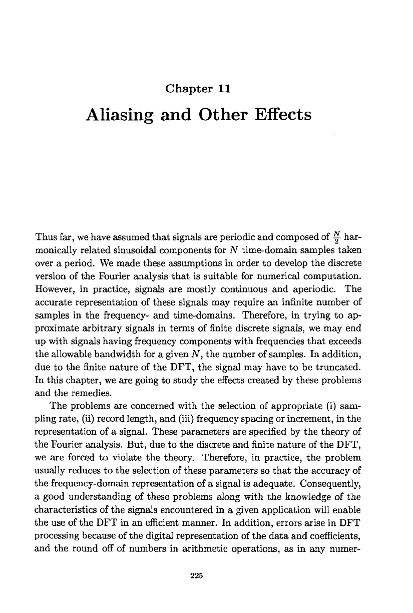
Fig. 11.1 (a) Significant magnitude of frequency components in an infinite range. Alias-

ing is unavoidable, (b) Nonzero value of frequency components only in a finite range.

Aliasing is avoidable by providing a sufficient frequency range, (c) Magnitude of fre-

quency components falls off as frequency increases. Aliasing can be made negligible by

an appropriate choice of the frequency range.

ical computation using digital devices. In Sec. 11.1, the aliasing effect is

described. In Sec. 11.2, the leakage effect is analyzed. In Sec. 11.3, the

picket-fence effect is explained.

11.1 Aliasing Effect

The theory of the Fourier analysis is that a periodic signal can be rep-

resented uniquely by a spectrum with an infinite number of harmonically

related sinusoids as shown in Fig. 11.1(a). Since we can deal with only a

finite number of frequency components in the DFT, we are faced with the

following two alternatives: (i) we can represent a signal uniquely with a fi-

nite number of frequency components if the signal is band-limited as shown

in Fig. 11.1(b) or (ii) we give up unique and unambiguous representation of

the signal. The DFT spectral representation of a signal will be in gross er-

ror due to aliasing if its spectrum is as shown in Fig. 11.1(a) (spectrum has

significant values up to infinity). Fortunately, in practice, the spectrum of

Aliasing Effect

227

signals tends to fall off to insignificant levels at high frequencies as shown in

Fig. 11.1(c) so that the error is within tolerable limits in the representation

of the signal with sinusoids whose frequencies span only a finite range.

In order to understand the problem of fixing the frequency range, we

want to get answers to two questions: (i) for a given N, what is the highest

frequency component present in a signal so that it can be unambiguously

represented by the DFT coefficients, and (ii) if a signal is composed of

frequency components of higher frequencies than that can be allowed for

its proper representation, what problem it creates and what are the possible

remedies to that problem.

The highest frequency component for unambiguous signal

representation

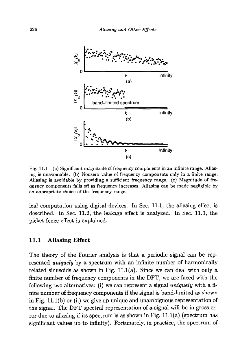
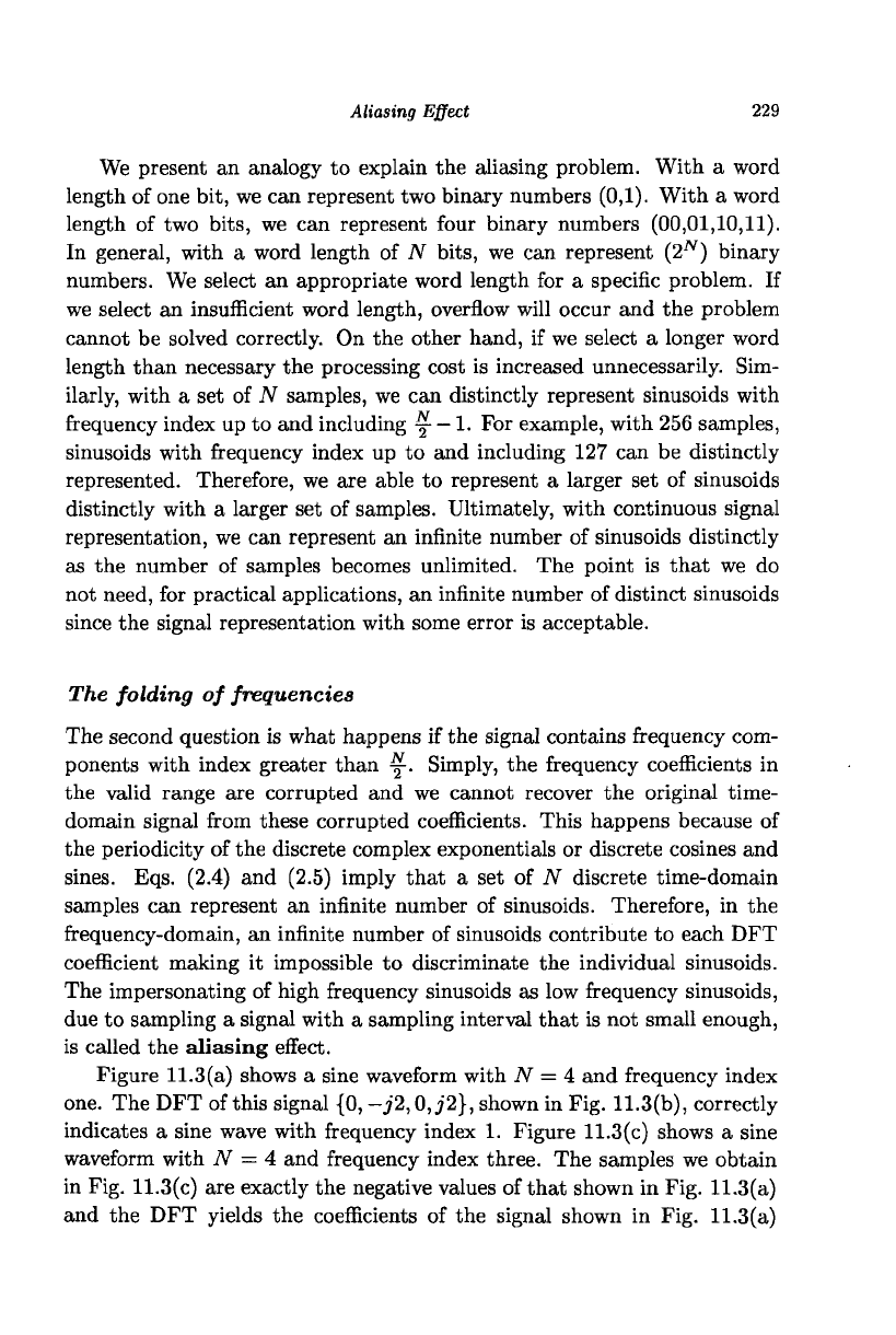
Let us assume that we use N = 4 samples to represent a signal. Fig-

ures 11.2(a) and (b) show, respectively, the representation of sine and co-

sine signals with zero frequency. Figures 11.2(c) and (d) show, respectively,

the representation of sine and cosine signals with frequency index one. The

set of samples, in each of these cases, is distinct and unambiguously repre-

sent the corresponding signal. Figures 11.2(e) and (f) show, respectively,

the representation of sine and cosine signals with frequency index two. A

cosine wave with frequency index two has a distinct set of samples and

can be unambiguously represented with four samples. The set of samples

in Figs. 11.2(a) and (e) are the same. Therefore, we cannot represent a

sine wave of frequency index two with four samples. If we use five samples

we could represent the sine wave with frequency index two unambiguously.

With two samples per cycle, the representation is not possible while just

more than an average of two samples per cycle is adequate. This implies

that the sampling rate or frequency must be greater than two times of

the frequency of the highest frequency component of a signal. That is, the

minimum number of samples required is two times the frequency index plus

one.

For example, with frequency index one, we need three samples. With

frequency index ~, we need

samples which exceeds our assumption of

N samples. Our conclusion is that the index of the highest frequency com-

ponent a signal is composed of must be less than y with N time-domain

samples, in order to represent the signal unambiguously with N DFT co-

efficients. This is called the sampling theorem and the frequency with

index y is called the folding frequency.

228 Aliasing and Other Effects

£ 0

(a)

(c)

(e)

* °

-1

4 0

(f)

Fig. 11.2 (a), (c), and (e): Sine waves with frequency indices 0, 1, and 2, respectively,

with 4 samples, (b), (d), and (f): Cosine waves with frequency indices 0, 1, and 2,

respectively, with 4 samples. Waveforms shown in (a), (b), (c), (d), and (f) only have

distinct set of sample values.

The conclusion we arrived is a theoretical answer to our first question.

In practice, due to the inability of physical devices to produce ideal behavior

as represented mathematically, typically the index of the highest frequency

component present in a signal is limited to ^ in order to represent the

signal in the frequency-domain with reasonable accuracy. This implies that

at the least four samples per cycle of a sinusoid are available. If the number

of samples per cycle is decreased, it results in more inaccuracy in the signal

representation. On the other hand, if we do have more than the necessary

number of samples per cycle then the computational effort for processing

the signal is increased unnecessarily. The number of samples per cycle, for

a practical problem, has to be determined considering both these aspects.

We have concluded that aliasing is avoided in the frequency-domain if

the sampling interval, T

, in the time-domain is less than ^ where fh is

the highest frequency of the component of a signal. Aliasing is avoided in

the time-domain if the sampling interval in the frequency-domain, f

, is

less than ^, where T is the record length of an aperiodic signal.

Aliasing Effect 229

We present an analogy to explain the aliasing problem. With a word

length of one bit, we can represent two binary numbers (0,1). With a word

length of two bits, we can represent four binary numbers (00,01,10,11).

In general, with a word length of N bits, we can represent (2^) binary

numbers. We select an appropriate word length for a specific problem. If

we select an insufficient word length, overflow will occur and the problem

cannot be solved correctly. On the other hand, if we select a longer word

length than necessary the processing cost is increased unnecessarily. Sim-

ilarly, with a set of N samples, we can distinctly represent sinusoids with

frequency index up to and including ^

!• F°

example, with 256 samples,

sinusoids with frequency index up to and including 127 can be distinctly

represented. Therefore, we are able to represent a larger set of sinusoids

distinctly with a larger set of samples. Ultimately, with continuous signal

representation, we can represent an infinite number of sinusoids distinctly

as the number of samples becomes unlimited. The point is that we do

not need, for practical applications, an infinite number of distinct sinusoids

since the signal representation with some error is acceptable.

The folding of frequencies

The second question is what happens if the signal contains frequency com-

ponents with index greater than %• Simply, the frequency coefficients in

the valid range are corrupted and we cannot recover the original time-

domain signal from these corrupted coefficients. This happens because of

the periodicity of the discrete complex exponentials or discrete cosines and

sines.

Eqs. (2.4) and (2.5) imply that a set of N discrete time-domain

samples can represent an infinite number of sinusoids. Therefore, in the

frequency-domain, an infinite number of sinusoids contribute to each DFT

coefficient making it impossible to discriminate the individual sinusoids.

The impersonating of high frequency sinusoids as low frequency sinusoids,

due to sampling a signal with a sampling interval that is not small enough,

is called the aliasing effect.

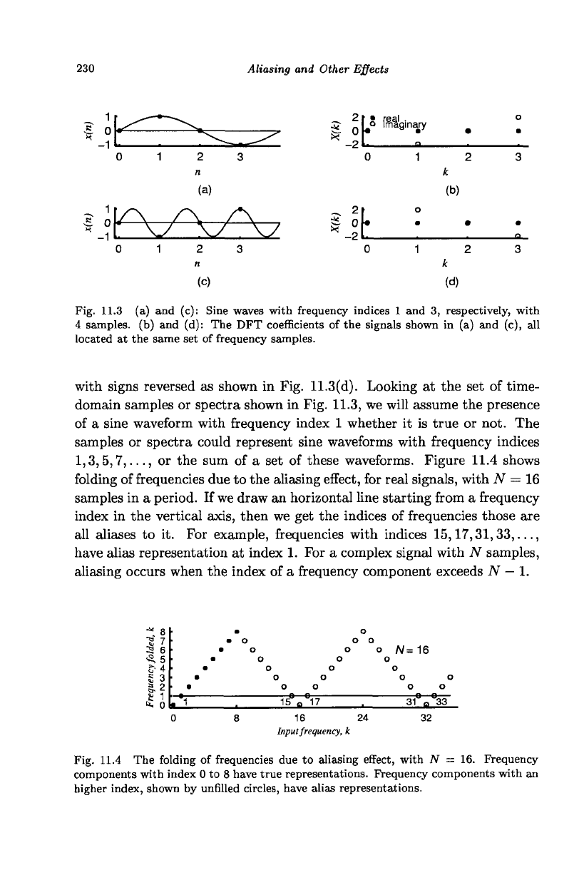
Figure 11.3(a) shows a sine waveform with N = 4 and frequency index

one.

The DFT of this signal {0,-j2,0,j2}, shown in Fig. 11.3(b), correctly

indicates a sine wave with frequency index 1. Figure 11.3(c) shows a sine

waveform with N = 4 and frequency index three. The samples we obtain

in Fig. 11.3(c) are exactly the negative values of that shown in Fig. 11.3(a)

and the DFT yields the coefficients of the signal shown in Fig. 11.3(a)

230

Aliasing and Other Effects

2 r

s pal

o Ima ginary

(a)

1 2

(b)

(c)

(d)

Fig. 11.3 (a) and (c): Sine waves with frequency indices 1 and 3, respectively, with

4 samples, (b) and (d): The DFT coefficients of the signals shown in (a) and (c), all

located at the same set of frequency samples.

with signs reversed as shown in Fig. 11.3(d). Looking at the set of time-

domain samples or spectra shown in Fig. 11.3, we will assume the presence

of a sine waveform with frequency index 1 whether it is true or not. The

samples or spectra could represent sine waveforms with frequency indices

1,3,5,7,...,

or the sum of a set of these waveforms. Figure 11.4 shows

folding of frequencies due to the aliasing effect, for real signals, with N — 16

samples in a period. If we draw an horizontal line starting from a frequency

index in the vertical axis, then we get the indices of frequencies those are

all aliases to it. For example, frequencies with indices 15,17,31,33,...,

have alias representation at index 1. For a complex signal with

samples,

aliasing occurs when the index of a frequency component exceeds N

—

•*. 8

•" 7

•2,5

S-4

3 •

a p .

»f r

6 1

". 0

o o

o o A/=16

o o

o o o

—e—e—

16 24

Input frequency, k

Fig. 11.4 The folding of frequencies due to aliasing effect, with N = 16. Frequency

components with index 0 to 8 have true representations. Frequency components with an

higher index, shown by unfilled circles, have alias representations.

Leakage Effect

231

Reducing the aliasing effect

In practice, aliasing will be present because if a signal is time-limited then

it cannot be band-limited and vice versa. Therefore, the aim is to reduce

it to allowable limits. One solution to reduce aliasing is to ensure that

the signal is composed of frequency components with index less than y

by prefiltering it with a low-pass filter. The second solution is to see that

the number of samples, N, is more than twice the index of the highest

frequency component present in the signal, if prior knowledge of the signal

is available. For example, high quality audio signals are band-limited to

about 20 kHz. For practical use, a sampling rate of 80 kHz is adequate. If

the highest frequency component of a signal is unknown, compute the DFT

of the signal with some arbitrary number of samples. Then, repeat the

process with double the number of samples, keeping the record length the

same. If the magnitudes of the DFT coefficients become negligible towards

the end of the spectrum (for real signals, close to the frequency with index

y),

then it is an indication that the value of N is sufficient. It may be

necessary to reduce the sampling interval further in order to reduce the

error due to aliasing created by the leakage effect described in the next

section.

11.2 Leakage Effect

In the last section, we considered the restriction on the range of frequencies

for the unique representation of a signal with a finite number of samples.

In this section, we consider the appropriate time-domain range over which

samples must be taken for the accurate representation of a signal. Again,

due to the finite nature of the DFT, we are forced to chop off some part

of the signal and hence we tend to violate the theory of Fourier analysis in

order to make the problem suitable for numerical analysis.

In the case of an aperiodic signal, since the period is infinity, we may

have to take samples over the entire time-domain range for the proper rep-

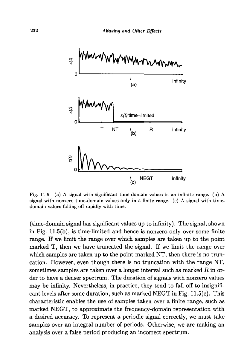
resentation of the signal. Figure 11.5(a) shows an aperiodic signal. In this

case,

in practice, we are forced to cutoff some part of the signal since only

a finite number of samples can be processed numerically. This is called

truncation and we represent only part of the signal correctly. Similar to

the case of the aliasing problem, the frequency-domain representation will

be in gross error due to truncation if the signal is as shown in Fig. 11.5(a)

232

Aliasing and Other Effects

^Hm^

(a)

infinity

#M^V

x(t) time-limited

T NT ' R

(b)

infinity

Fig. 11.5 (a) A signal with significant time-domain values in an infinite range, (b) A

signal with nonzero time-domain values only in a finite range, (c) A signal with time-

domain values falling off rapidly with time.

(time-domain signal has significant values up to infinity). The signal, shown

in Fig. 11.5(b), is time-limited and hence is nonzero only over some finite

range. If we limit the range over which samples are taken up to the point

marked T, then we have truncated the signal. If we limit the range over

which samples are taken up to the point marked NT, then there is no trun-

cation. However, even though there is no truncation with the range NT,

sometimes samples are taken over a longer interval such as marked R in or-

der to have a denser spectrum. The duration of signals with nonzero values

may be infinity. Nevertheless, in practice, they tend to fall off to insignifi-

cant levels after some duration, such as marked NEGT in Fig. 11.5(c). This

characteristic enables the use of samples taken over a finite range, such as

marked NEGT, to approximate the frequency-domain representation with

a desired accuracy. To represent a periodic signal correctly, we must take

samples over an integral number of periods. Otherwise, we are making an

analysis over a false period producing an incorrect spectrum.

Leakage Effect

233

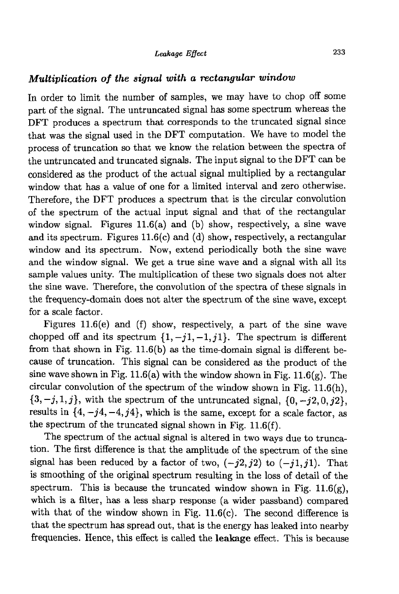
Multiplication of the signal with a rectangular window

In order to limit the number of samples, we may have to chop off some

part of the signal. The untruncated signal has some spectrum whereas the

DFT produces a spectrum that corresponds to the truncated signal since

that was the signal used in the DFT computation. We have to model the

process of truncation so that we know the relation between the spectra of

the untruncated and truncated signals. The input signal to the DFT can be

considered as the product of the actual signal multiplied by a rectangular

window that has a value of one for a limited interval and zero otherwise.

Therefore, the DFT produces a spectrum that is the circular convolution

of the spectrum of the actual input signal and that of the rectangular

window signal. Figures 11.6(a) and (b) show, respectively, a sine wave

and its spectrum. Figures 11.6(c) and (d) show, respectively, a rectangular

window and its spectrum. Now, extend periodically both the sine wave

and the window signal. We get a true sine wave and a signal with all its

sample values unity. The multiplication of these two signals does not alter

the sine wave. Therefore, the convolution of the spectra of these signals in

the frequency-domain does not alter the spectrum of the sine wave, except

for a scale factor.

Figures 11.6(e) and (f) show, respectively, a part of the sine wave

chopped off and its spectrum {1,

—jl,—l,jl}.

The spectrum is different

from that shown in Fig. 11.6(b) as the time-domain signal is different be-

cause of truncation. This signal can be considered as the product of the

sine wave shown in Fig. 11.6(a) with the window shown in Fig. 11.6(g). The

circular convolution of the spectrum of the window shown in Fig. 11.6(h),

{3)-J, Ijj}, with the spectrum of the untruncated signal, {0,-j'2,0,

j2},

results in {4, ~j4, -4,

j4},

which is the same, except for a scale factor, as

the spectrum of the truncated signal shown in Fig. 11.6(f).

The spectrum of the actual signal is altered in two ways due to trunca-

tion. The first difference is that the amplitude of the spectrum of the sine

signal has been reduced by a factor of two,

(-J2J2)

to (-jl,jl). That

is smoothing of the original spectrum resulting in the loss of detail of the

spectrum. This is because the truncated window shown in Fig. 11.6(g),

which is a filter, has a less sharp response (a wider passband) compared

with that of the window shown in Fig. 11.6(c). The second difference is

that the spectrum has spread out, that is the energy has leaked into nearby

frequencies. Hence, this effect is called the leakage effect. This is because