Sundararaja D. The Discrete Fourier Transform. Theory, Algorithms and Applications

Подождите немного. Документ загружается.

114

Fundamentals of the PM DFT Algorithms

the computation of odd indexed DFT vectors, odd subscripted input vector

elements combine to produce the new set of input vectors of one-half the

number.

The 2x1 PM DIF DFT algorithm

The basis of this type of algorithms is to divide the DFT vectors into two

groups and compute the values of these groups with reduced computation.

Since we divide the problem by partitioning the DFT vectors, this type of

algorithms is called decimation-in-frequency (DIF) algorithms.

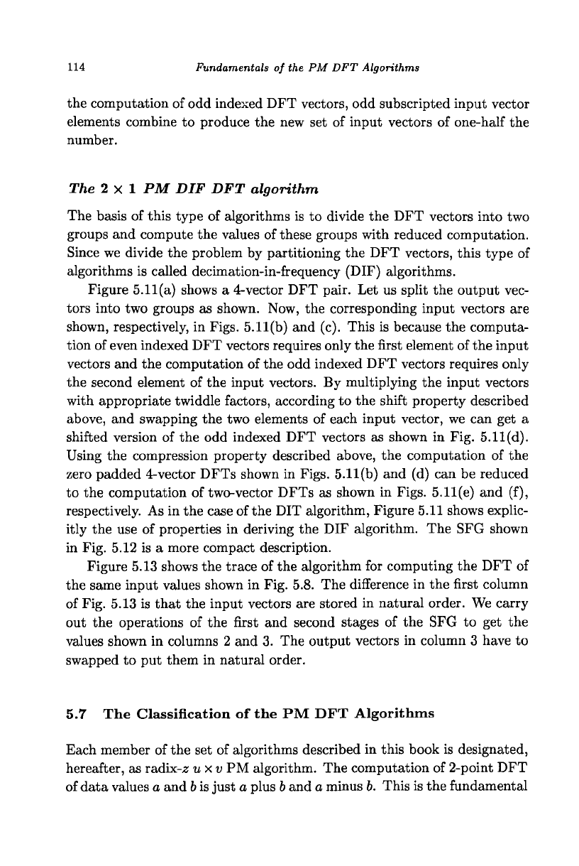
Figure 5.11(a) shows a 4-vector DFT pair. Let us split the output vec-

tors into two groups as shown. Now, the corresponding input vectors are

shown, respectively, in Figs. 5.11(b) and (c). This is because the computa-

tion of even indexed DFT vectors requires only the first element of the input

vectors and the computation of the odd indexed DFT vectors requires only

the second element of the input vectors. By multiplying the input vectors

with appropriate twiddle factors, according to the shift property described

above, and swapping the two elements of each input vector, we can get a

shifted version of the odd indexed DFT vectors as shown in Fig. 5.11(d).

Using the compression property described above, the computation of the

zero padded 4-vector DFTs shown in Figs. 5.11(b) and (d) can be reduced

to the computation of two-vector DFTs as shown in Figs. 5.11(e) and (f),

respectively. As in the case of the DIT algorithm, Figure 5.11 shows explic-

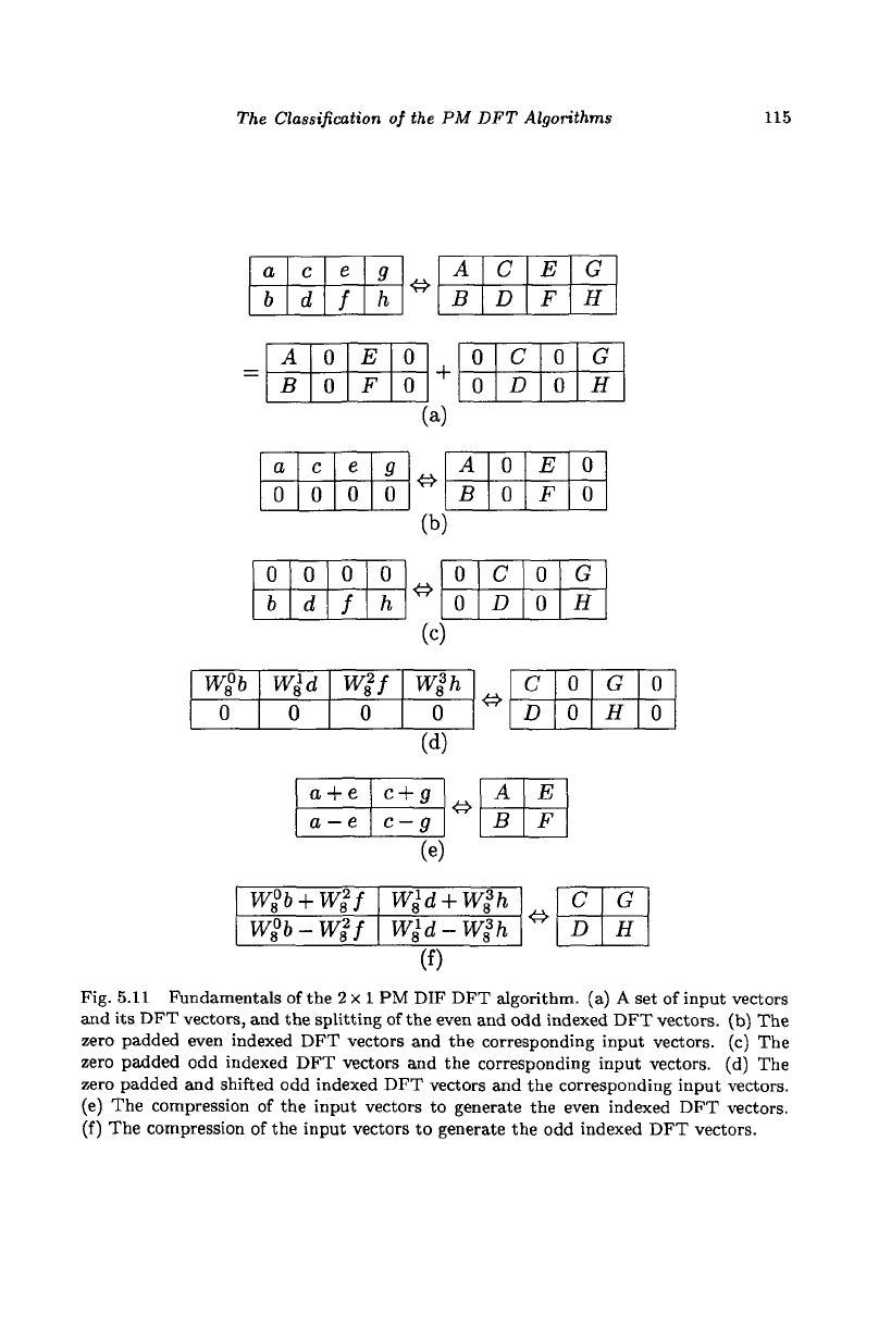
itly the use of properties in deriving the DIF algorithm. The SFG shown

in Fig. 5.12 is a more compact description.

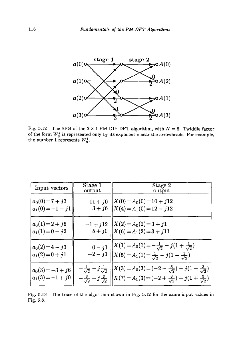
Figure 5.13 shows the trace of the algorithm for computing the DFT of

the same input values shown in Fig. 5.8. The difference in the first column

of Fig. 5.13 is that the input vectors are stored in natural order. We carry

out the operations of the first and second stages of the SFG to get the

values shown in columns 2 and 3. The output vectors in column 3 have to

swapped to put them in natural order.

5.7 The Classification of the PM DFT Algorithms

Each member of the set of algorithms described in this book is designated,

hereafter, as radix-z uxv PM algorithm. The computation of 2-point DFT

of data values a and

is just a plus

and a minus b. This is the fundamental

The Classification of the PM DFT Algorithms

115

(a)

<£•

(b)

(c)

W$b

Wid

wif

Wih

(d)

a +

—

c-9

(e)

Wib

Wif

W§b-

Wif

Wih

Wid-Wih

(f)

Fig. 5.11 Fundamentals of the 2 x 1 PM DIF DFT algorithm, (a) A set of input vectors

and its DFT vectors, and the splitting of the even and odd indexed DFT vectors, (b) The

zero padded even indexed DFT vectors and the corresponding input vectors, (c) The

zero padded odd indexed DFT vectors and the corresponding input vectors, (d) The

zero padded and shifted odd indexed DFT vectors and the corresponding input vectors.

(e) The compression of the input vectors to generate the even indexed DFT vectors.

(f) The compression of the input vectors to generate the odd indexed DFT vectors.

116

Fundamentals of the PM DFT Algorithms

Fig. 5.12 The SFG of the 2 x 1 PM DIF DFT algorithm, with N = 8. Twiddle factor

of the form Wg is represented only by its exponent s near the arrowheads. For example,

the number 1 represents Wg.

Input vectors

(0) = 7+j3

ai(0) = -l-jl

(l) =

+ j6

(l)=0-j2

(2)=4-j3

(2)=0+jl

(3) = -3+j6

ai(3) = -l+j0

Stage 1

output

11+JO

3+J6

-1+J12

5+jO

0-jl

-2-jl

_ 3 _ -• 3

Stage 2

output

X(0) = Ao(0) =

+ jl2

X(4) = Ai{0) =

- jl2

X(2) =

(2)

= 3 + jl

X(6)=Ai(2) =

+ jll

X(l) = A

(l) = -^-j(l + ^)

X(3) =

(3)

= (-2- ^) - j(l- ^)

X(7)=A

(3) = (-2+ ±) - j(l + ^)

Fig. 5.13 The trace of the algorithm shown in Fig. 5.12 for the same input values in

Fig. 5.8.

Summary

117

operation in the algorithm. Hence, the name plus-minus (PM). The term

radix-z specifies the way a problem is decomposed into smaller problems.

While we can design algorithms with any radix, the practically most useful

value for z is two and, therefore, the algorithms described in this book are

exclusively of the type radix-2. In a radix-2 algorithm, a problem is split

into two smaller independent problems of the same type, each of half the

size,

recursively from the input or output end. The solutions of two smaller

problems are combined to form the solution of a larger problem. A radix-2

algorithm requires that the length of the data N divided by the vector

length u is equal to an integral power of 2, that is ^ = 2

where m is an

integer.

The letter u indicates the number of elements in a vector. Although

general expressions are developed in the following chapter, with one excep-

tion for vector length six, all the algorithms described, in detail, in this

book use a vector length of two since that length is practically the most

useful. It is possible to combine fully or partially the multiplication opera-

tions of two or more consecutive stages of an algorithm in order to reduce

the total number of arithmetic operations. However, the partial merging

of multiplication operations of adjacent stages leads to practically ineffi-

cient and irregular algorithms. Therefore, the letter v, in the range 1 to

m = log

—, specifies the number of adjacent stages whose multiplications

are combined. Although the set of PM algorithms is quite large, the prac-

tically more useful algorithms are those with z = 2, u — 2, and v = 1 or

v = 2. A good understanding of these algorithms will enable the reader to

derive algorithms with other parameters, if necessary.

5.8 Summary

• The problem of computing the DFT of N values is the problem of

evaluating N sums, each of N products. The challenge in designing

fast algorithms is to find the way to develop partial results and share

each partial result to compute as many coefficients as possible.

• The problem of computing the DFT can also be considered as the

decomposition of a larger DFT into smaller DFTs and combining

the coefficients of the smaller DFTs to produce the coefficients of

the larger DFT.

• In this chapter, the DFT and IDFT definitions using vector inputs

118

Fundamentals of the PM DFT Algorithms

and outputs were derived. The computation of the IDFT using the

DFT was presented. The fundamental principles and the relevant

theorems on which the fast algorithms are based were explained.

The classification of PM DFT algorithms was presented. In the

next few chapters, the PM DFT algorithms will be described in

detail.

References

(1) Sundararajan, D., Ahmad, M. O. and Swamy, M. N. S. (1994)

"Computational Structures for Fast Fourier Transform Analyzers",

U.S. Patent, No. 5,371,696.

(2) Sundararajan, D., Ahmad, M. O. and Swamy, M. N. S. (1998)

"Vector Computation of the discrete Fourier Transform", IEEE

Trans. Cir. and Sys. II, vol. CAS-45, No.4, pp.

449-461.

Exercises

5.1 Using the SFG shown in Fig. 5.1, compute the DFT of:

5.1.1.

x(n) =

{2,3,5,4}.

* 5.1.2. x(n) = {2+jl,l-j2,2 + j2,l-j3}.

5.2 Starting from the DFT definition, derive the expression Eq. (5.7) with

N = 8.

5.3 Starting from the IDFT definition, derive the expression Eq. (5.11)

with N = 8.

5.4 Using the SFG shown in Fig. 5.3, compute the IDFT of

X(k) = {2-jl,l-j2,3 + j2,l-j3}.

* 5.5 Using the SFG shown in Fig. 5.4, compute the IDFT of

X(k) = {2 - jl,

- j2,3 + j2,1 - j3} using DFT.

5.6 Verify that the transform vectors shown in Fig. 5.5(d) corresponds to

the input vectors shown in Fig. 5.5(c).

5.7 Compute the input vectors, {a

(0), a

(l)}, with vector length 2 if

x(n) = {1 - j4,2 + j3,1 - jl, 2 - jl}. Find the DFT using the vectors.

Deduce the DFT if the input vectors are {a

(0),0,a

(l),0}.

Exercises 119

5.8 Using the SFG shown in Fig. 5.7, compute the DFT of x(n) = {1 -

j4,2-j3,l-jl,2-j4,2-j2,l+j3,l-jl,2 + j2}.

* 5.9 Using the SFG shown in Fig. 5.7, compute the IDFT of X(k) =

{l-j3,2-j3,3-jl,2-j4,3 + j3,2-j2,l +

j3,2+;4}.

* 5.10 Using the SFG shown in Fig. 5.12, compute the DFT of x(n) =

{1 - jA, 2 - j3,1 - jl,

- j4,2 - j2,1 + j3,1 - jl, 2 + j2}.

5.11 Using the SFG shown in Fig. 5.12, compute the IDFT of X(k) =

{l-j3,2-j3,3-jl,2-j4,3 + j3,2-j2,l + j3,2 + j4}.

Programming Exercise

5.1 Write a program to directly implement Eq. (5.7) to compute the DFT.

Chapter 6

The u X 1 PM DFT Algorithms

The problem of computing the DFT is multiplication of the data with

samples of complex exponentials of various frequencies and summing it up.

In the direct computation of the defining equation, the multiplication and

addition operations required to determine each frequency coefficient are

carried out separately. In fast computation of the DFT, the multiplication

and addition operations are carried out in parts over several stages. This

spreading of the computation makes it possible to compute partial results

and use them for the computation of several frequency coefficients. In the

last chapter, we derived the vector form of the DFT definition. In addition,

fast DIT and DIF algorithms, for small values of N, were developed using

the basic principles. In this chapter, we will study more formally the class

of algorithms in which the computation is split over several stages without

merging the multiplication operations of adjacent stages.

The general version of the u x 1 PM DIT DFT algorithms is derived in

Sec.

6.1. Then, we deduce the DIT algorithm for the most efficient vector

length u = 2 and give a detailed description in Sec. 6.2. The necessity

of reordering the input vectors for in-place computation is explained in

Sec.

6.3. In Sec. 6.4, the computation of a single DFT coefficient is traced

in the SFG of the algorithm. The general version of the uxl PM DIF

DFT algorithms is derived in Sec. 6.5. The 2 x 1 PM DIF DFT algorithm

is deduced in Sec. 6.6. The computational complexity of the 2x1 PM DFT

algorithms is presented in Sec. 6.7. The 6 x 1 PM DIT DFT algorithm,

which provides the computation of DFT for lengths with a factor of three,

is described in Sec. 6.8. A flow chart description of the 2 x 1 PM DIT DFT

algorithm is given in Sec. 6.9.

121

122

The uxl PM DFT Algorithms

6.1 The uxl PM DIT DFT Algorithms

Decomposing the summation in Eq. (5.4) into those corresponding to the

even and odd indexed input values a

(n) and simplifying, we get

M. _,

•3,1

/•nk

Mk)= Y,

(2n)Wf

n=0

+ W*W% J2

(2n

+ l)Wf, (6.1)

n=0

where q = ((k + p^-) mod u), p =

0,1,...,

—

1, and

0,1,..., —

—

The DFT values A

(k + ^), k =

0,1,...,

^ - 1, can be obtained by

replacing k with

+ ^ in Eq. (6.1). The resulting equation can be written

(k+^)

= £

(2n)WZ

71=0

-Nil

+ WZWl

Wk Y, W£*>

{2n + l)W£, (6.2)

n=0

where q = ((k+ £j+pf) mod u), p =

0,1,...,u-1,

and k =

0,1,..., ^-1.

Let the DFT of the even indexed input vector elements, a

(n),n =

0,2,..., ^-2, be represented by Ay (k), and that of the odd indexed input

vector elements, a

(n), n —

1,3,...,

—

1, be represented by Ay(k). For

even indexed input vectors,

4*)(fc)= Y Wra

{2n)W£

where q = ((A; + p^) mod u), p

— 0,1,...,

—

1, and k =

0,1,...,

—

For even values of p, as Ay (k) is periodic of period u with respect to the

variable p,

4?mod„(*) = £

W^a

{2n)Wf,

Theuxl PM DIT DFT Algorithms

123

where q = ((fc + p%) mod u), p =

0,1,...,

u - 1, and fc =

0,1,...,

^~ - 1.

For odd values of p,

i) „.„«(*>

^^"a^Wf,

n=0

where 9 = ((fc+P^ + ^) mod u), p =

0,1,...

,«-l, and fc =

0,1,..., ^-1-

Similarly, for odd indexed input vectors, for even values of p,

4?mod«(*)= E ^i

2p)

"^(2n + l)Wf,

where g = ((fc + p^) mod u), p =

0,1,...,

u - 1, and fc =

0,1,...,

^ - 1.

For odd values of p,

ra=0

where g= ((fc+P^ + ^j) modu),p =

0,1,..

.,u-l, and fc =

0,1,..., ^-1.

Equations (6.1) and (6.2), using the smaller size DFTs defined above,

can be written as

Mk) = A

mo<i

uW +

WSW^A{

modu

(k)

(6.3)

(k+^)

= <

+1)modu

(fc)+^^^^

+1)modu

(fc),(6.4)

where p =

0,1,...,

u - 1 and fc =

0,1,...,

|£ - 1. The problem of comput-

ing an ——vector DFT has been decomposed into a problem of computing

two ^—vector DFTs. This process of decomposition can be continued

recursively, until the problem is reduced to a set of

1-vector

DFTs.

The u X 1 PM DIT DFT butterfly

As the DFT of a single vector is

itself,

we never compute the DFT of a set

of vectors using the definition. Therefore, the process, which is repeated

several times over a number of stages, is only the decomposition of a larger

DFT into two smaller DFTs. The basic computation that is repeatedly

used in the decomposition process is called the butterfly computation.

In general, the butterfly computation at the rth stage, for an even vector

length (For an odd vector length, the first and third equations of Eq. (6.5)