Sundararaja D. The Discrete Fourier Transform. Theory, Algorithms and Applications

Подождите немного. Документ загружается.

104

Fundamentals of the PM DFT Algorithms

The sum of these yields a;(fe) and difference yields x(k +

—•).

The access of

correct twiddle factor values is carried out using the mod function. Inside

the inner loop, the coefficient computation is carried out according to the

DFT definition. The next module, shown in Fig. 5.2(e) prints the real and

imaginary parts of the DFT values, respectively, from the arrays xr and xi,

one complex coefficient in each iteration. This module is called out-put.

5.3 Vector Format of the IDFT

A set of expressions similar to those given by Eqs. (5.5), (5.6), and (5.7)

can be obtained for computing the IDFT.

B(k) = {B

(k),B

(k)} = {X(k) + X(k+j),X{k)-X(k+^)},

* = 0,l,...,y-l (5.9)

b(n) = {b

(n),b

(n)} = {x(n),x(n+j)}, n =

0,1,...,

y - 1 (5.10)

M«) = ^£(-l)

*^(*W

*, n = 0,l,...,y-l (5.11)

fc=0

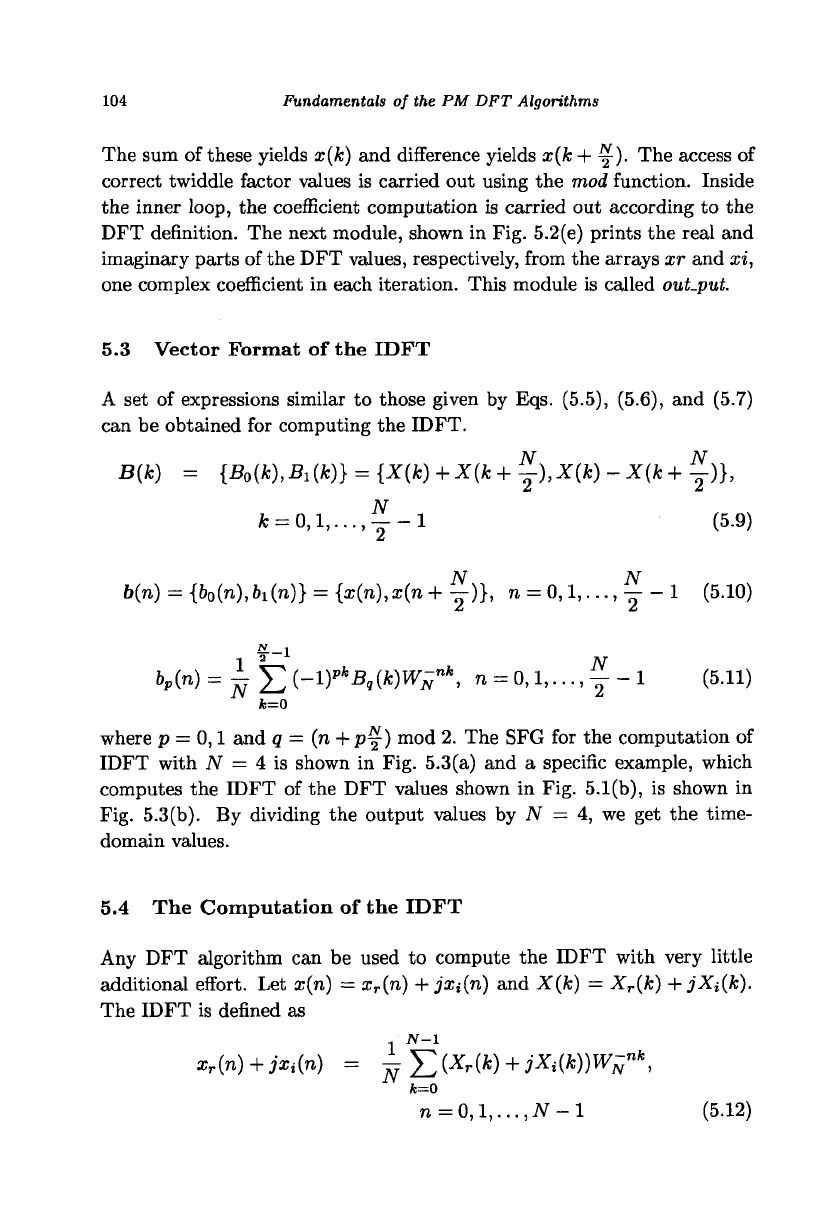
where p = 0,1 and q = (n + py) mod 2. The SFG for the computation of

IDFT with TV = 4 is shown in Fig. 5.3(a) and a specific example, which

computes the IDFT of the DFT values shown in Fig. 5.1(b), is shown in

Fig. 5.3(b). By dividing the output values by N = 4, we get the time-

domain values.

5.4 The Computation of the IDFT

Any DFT algorithm can be used to compute the IDFT with very little

additional effort. Let x{n) — x

{n) + jxi(n) and X(k) = X

(k) + jXi(k).

The IDFT is defined as

N-l

(n)+jxi(n) = ^Y^

) +

3Uk))W^

n = 0,l,...,JV-l (5.12)

k=0

The Computation of the IDFT

105

B(0)={B

(0),

(0) }= cv » MWMbo

(0),

h (0)}={ar(0), x(2)})

{X{0)+X(2),X(0)-X(2)} X/*" 46

(0) = B

(0) + B

(l)

(0) = flo(0)-B

(l)

B(1)={B

(1), Bj.(1)}= </ > ^b4(ft(l)={b

(l), 6

(l)}={ar(l), x(3)})

{X(1)+X(3),X(1)-X(3)} 4fe

(l) = B

(0) + W

(l)

(a)

(l) = 5

(0)-W7

Bi(l)

(8 + j4)±(4 + j2)=

o^—^^{8

+ j4,16 + j8}

{12+j6,4 + j2}

(-5 - j5) ± (1 + j3) = c^ ^ {12 - j4, -4 + j8}

{-4-A-6-J8}

(b)

Fig. 5.3 (a) The SFG for the computation of 4-point IDFT. (b) A specific example of

(a) for computing the IDFT of the DFT values in Fig. 5.1(b).

By conjugating both sides, we obtain

JV_1

(n)

= T7 E ^(

) - 3Xi(k))Wp (5.13)

k=0

Equation (5.13) represents a DFT with the input and output data conju-

gated, in addition to a constant divisor. This implies that a DFT algorithm

can be used to compute the IDFT by conjugating the input, computing the

DFT, and conjugating the output. An alternate algorithm is obtained by

multiplying both sides of Eq. (5.13) by j.

N-l

Xi{n) +

(n) = - J2 (Xi(k) +jX

(k))Wtf

(5.14)

fc=0

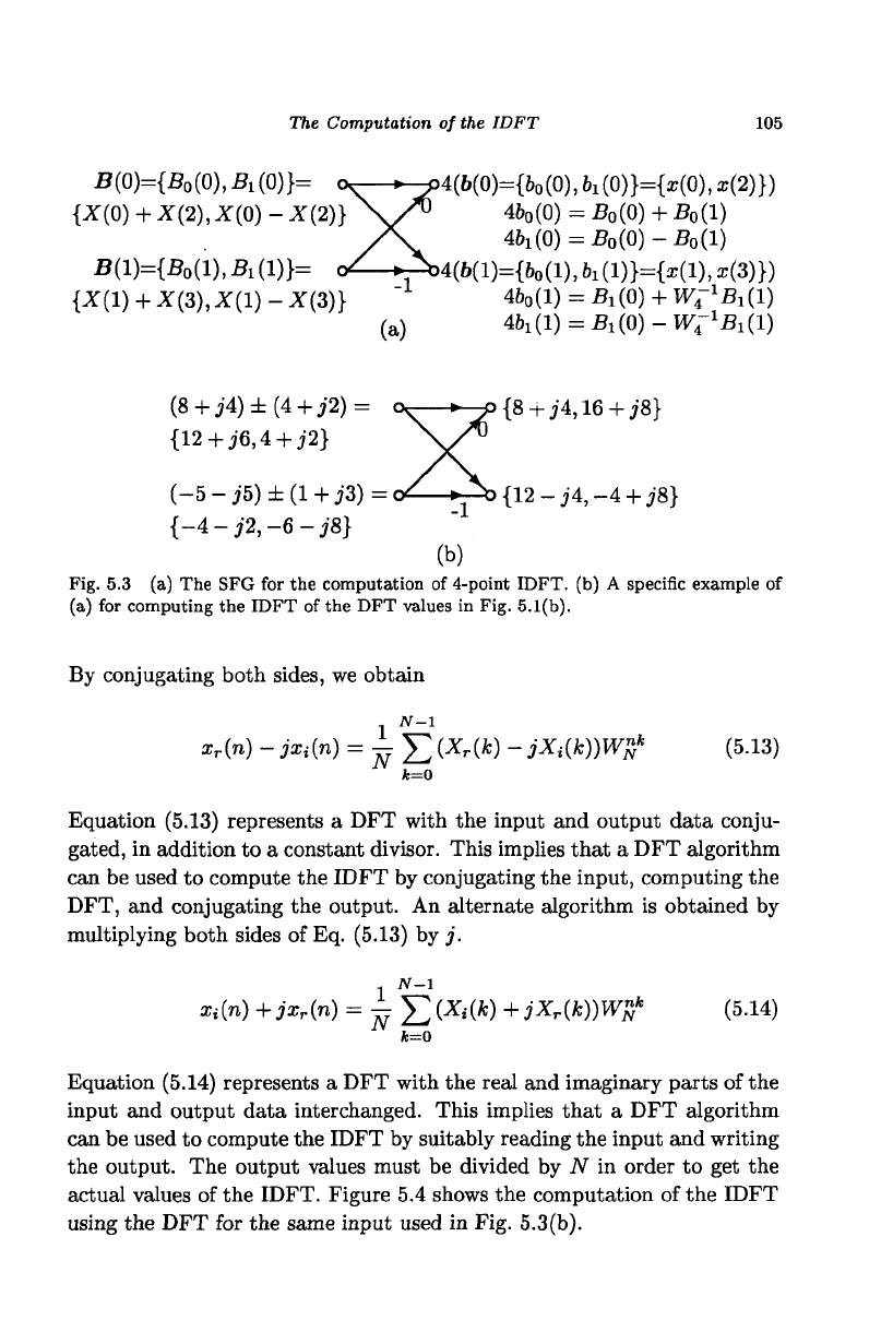
Equation (5.14) represents a DFT with the real and imaginary parts of the

input and output data interchanged. This implies that a DFT algorithm

can be used to compute the IDFT by suitably reading the input and writing

the output. The output values must be divided by N in order to get the

actual values of the IDFT. Figure 5.4 shows the computation of the IDFT

using the DFT for the same input used in Fig. 5.3(b).

106

Fundamentals of the PM DFT Algorithms

{6 + jl2,2+j4}

<v »

p{4

8;8

jl6}

{-2-j4,-8-j6}o/

>\{-4

jl2,8-j4}

Fig. 5.4 A specific example of computing 4-point IDFT of the DFT values in Fig. 5.1(b)

using the DFT.

5.5 Fundamentals of the PM DIT DFT Algorithms

Efficient DFT algorithms are obtained by decomposing Eq. (5.4) into sev-

eral stages of computation. In this section, we derive the DIT type of algo-

rithms. In order to do that, we have to study two properties on which this

type of algorithms is based. For simplicity, we will develop the algorithm

for the specific case with N = 8 and u = 2.

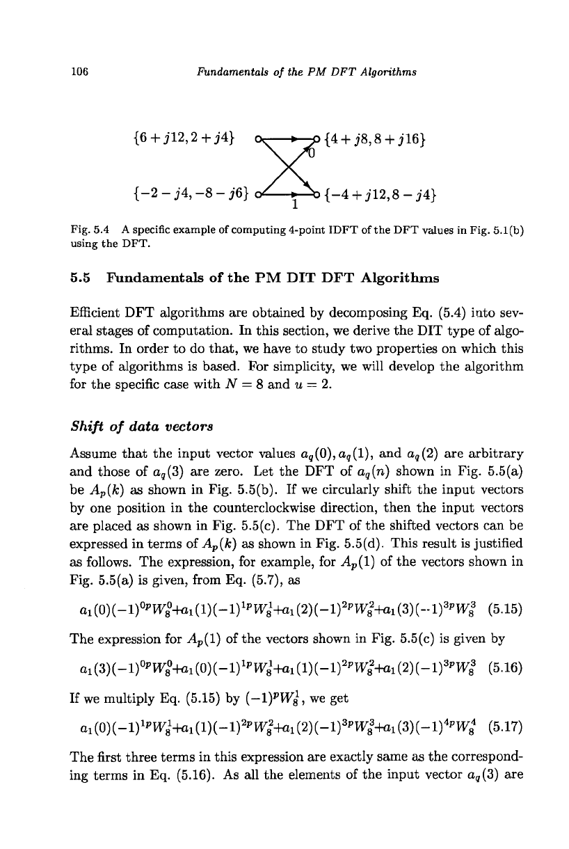
Shift of data vectors

Assume that the input vector values a

(0),a

(l), and o,(2) are arbitrary

and those of a

(3) are zero. Let the DFT of a

(n) shown in Fig. 5.5(a)

be A

(k) as shown in Fig. 5.5(b). If we circularly shift the input vectors

by one position in the counterclockwise direction, then the input vectors

are placed as shown in Fig. 5.5(c). The DFT of the shifted vectors can be

expressed in terms of A

(k) as shown in Fig. 5.5(d). This result is justified

as follows. The expression, for example, for A

(l) of the vectors shown in

Fig. 5.5(a) is given, from Eq. (5.7), as

ai(0)(-l)°W

°4<

(l)(-l)

(2)(-l)

(3)(-l)

(5.15)

The expression for A

{1) of the vectors shown in Fig. 5.5(c) is given by

Oi(3)(-l)

°+a

(0)(-l)

(l)(-l)

^i(2)(-l)

(5.16)

If we multiply Eq. (5.15) by (-1)

, we get

^^(-^^^^(^(-^^^(^(-^^^^(^(-l)^^

(5.17)

The first three terms in this expression are exactly same as the correspond-

ing terms in Eq. (5.16). As all the elements of the input vector a

(3) are

Fundamentals of the PM DIT DFT Algorithms 107

a,(l) A

(l)

• •

a„(2)« a

(n) • a

(0) A

(2)» A

(k) • A

{0)

(3) = 0 A

{3)

(a) (b)

(0)

W%W£A

(1)

(l)« a

(n-l) • a

(3) W

(2). WiW

(k) •WfW§A

(p)

= 0

o,(2)

W%WiA

(3)

Fig. 5.5 (a) A set of

input vectors with the last vector having all zero elements and (b)

its DFT. (c) The shifted vectors of (a) by one position in the counterclockwise direction

and (d) its DFT in terms of the DFT vectors shown in (b).

zero,

the term involving this vector does not contribute to the summation.

Therefore, Eqs. (5.16) and (5.17) yield the same value.

Zero padding of data vectors

Assume that we zero pad a set of ^ input vectors by inserting vectors with

all zero elements in between two vectors to get a set of ^ input vectors.

Then, the DFT of the new set of input vectors is defined as

(

) = E Wra

(n)W?*, k =

0,1,...,

n=0

108

Fundamentals of the PM DFT Algorithms

Since the odd indexed input vectors are zero, we get

(

) = E Wf

(2n)WZ

, k =

0,1,...,

^ - 1

n=0

Now, for k =

0,1,...,

—

- 1, we get

T7-1

(k)

p)na

<>(

)

n=0

R,r*=£,£ + l,...,2£-l,weget

A^{k)

= Y, Wgv+V

(2n)W%

rnk

n=0

Since A

(k) is periodic of period u with respect to the variable p, we get

A^{k)

= A

{2p) mod u

(k), A^(k + —) = Apjp+i)

od «(*),

p =

0,1,..

.,u

—

1, fc =

0,1,...,

For an even vector length, when the number of input vectors is doubled

by inserting vectors with all zero elements in between the vectors, the even

subscripted vector elements of the smaller DFT repeat for the first-half of

the DFT of the zero padded input vectors and the odd subscripted DFT

vector elements repeat for the second

half.

For example,

{(a,b),(e,f)}&{(A,B),(E,F)}

implies

{(a,b),{0,0),(e,f),(0,0)}^{(A,A),(E,E),(B,B),(F,F)}

The 2x1 PM DIT DFT algorithm

The naming of the algorithm will be explained at the end of this chapter.

The basis of this type of algorithms is to divide the computation into the

computation of the DFTs of the even and the odd indexed input vectors.

These DFTs are then combined to form the required DFT. Because the

time-domain vectors are divided into two smaller groups, this approach

is called decimation-in-time (DIT). For example, in order to compute the

DFT of four input vectors, the input vectors are split into two groups of

Fundamentals of the PM DIT DFT Algorithms

109

(a)

(b)

(c)

•&

w°c

-w$c

W^G

-WIG

WiD

-WiD

WiH

-WiH

(d)

wic

-wic

W£G

-WIG

WiD

-WiD

WiH

-WiH

A + WiC

A - WiC

E + W£G

E - W£G

(e)

B + WiD

B - WiD

F + WiH

F - WiH

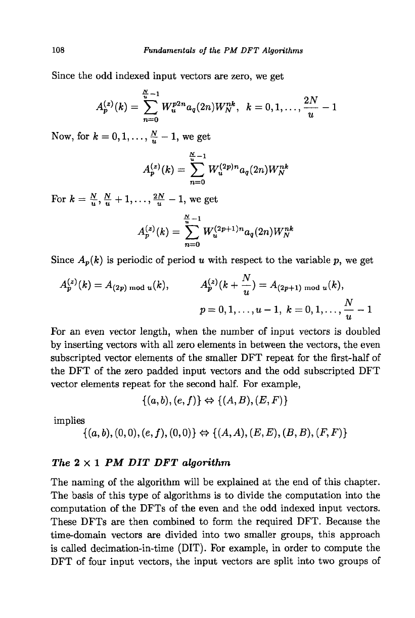
Fig. 5.6 Fundamentals of the 2 x 1 PM DIT DFT algorithm, (a) The DFT of the even

and odd indexed input vectors in (e). (b) The DFT of the zero padded even indexed

input vectors, (c) The DFT of the zero padded odd indexed input vectors, (d) The DFT

of zero padded and shifted odd indexed input vectors, (e) The DFT of 4 input vectors

is obtained as the sum of the DFTs of zero padded even and odd indexed input vectors.

zero padded even and odd indexed vectors as shown in Fig. 5.6(e). The sum

of the two groups of the input vectors is equal to the given input vectors. If

we compute the DFT of the two groups of input vectors and add, due to the

linearity property of the DFT, we get the DFT of the given input vectors.

Note that, due to zero padding, the computation of the DFT of each group

of vectors can be reduced to the computation of a 2-vector DFT.

Consider the DFT vector pairs shown in Fig. 5.6(a). Due to zero padding

110 Fundamentals of the PM DFT Algorithms

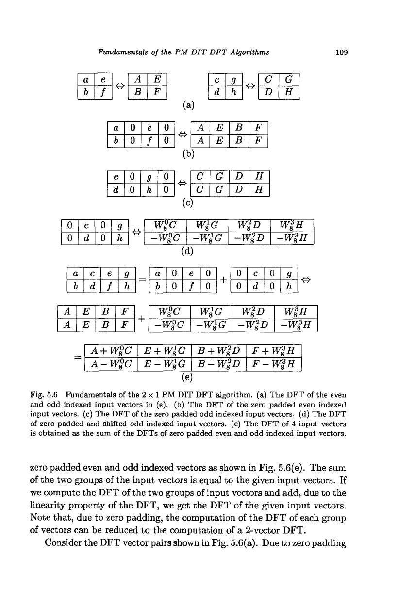
Fig. 5.7 The SFG of the 2 x 1 PM DIT DFT algorithm, with N = 8. Twiddle factor of

the form Wg is represented only by its exponent s near the arrowheads. For example,

the number 1 represents Wg.

property described above, we can deduce the DFT of the vectors shown

on the left side of Figs. 5.6(b) and (c) as shown on the right side. The

DFT of the shifted input vectors shown in Fig. 5.6(d) can be obtained by

multiplying the DFT vectors shown in Fig. 5.6(c) with appropriate twiddle

factors. Due to the linearity property of the DFT, the sum of the DFTs

shown in Figs. 5.6(b) and (d) is the DFT of the sum of the input vectors

shown in those figures. The point is that we are able to compute a longer

DFT (a 4-vector DFT) by combining the coefficients of two 2-vector DFTs

as shown in Fig. 5.6(e).

The SFG of the 2 x 1 PM DIT DFT algorithm is shown in Fig. 5.7. Note

that the computation module shown, with N = 4, in Fig. 5.1 is used four

times,

with N = 8. We will say more about the structure of the SFG in

the next few chapters. While Figs. 5.6 and 5.7 depict the same algorithm,

the SFG shown in Fig. 5.7 is a more compact description whereas Fig. 5.6

shows explicitly the use of properties in deriving the algorithm.

In order to understand the algorithm, let us use an algorithm trace. A

trace of an algorithm is a table of values of the variables at various stages

of the algorithm from input to output. Figure 5.8 shows the trace of the

algorithm shown in the SFG of Fig. 5.7. The input data is {x(n),n =

0,1,2,3,4,5,6,7} = {3 + jl,l+j2,2-jl,-2 + j3,4 + j2,l + j4,2-

j2,

—1

+ j3}. With N = 8 and u = 2, four vectors are required and the

input values are read into the vector locations as shown in column 1. For

example, a;(0) = 3+jl and x(4) = 4+j2 are stored in the storage locations

of the first vector. Vector formation consists of computing 2-point DFT

of the values stored in each vector locations. For example, the first vector

Fundamentals of the PM DIT DFT Algorithms

111

Input values

stored in vector

locations

x(0)=3+jl

z(4)=4+j2

x{l)=l+j2

x(5)=l+j4

x(2)=2-jl

x(6)=2-j2

x(3)=-2+j3

ar(7)=-l+j3

Vector

formation

and swapping

(0)=7+;3

oi(0)=-l-jl

(2)=4-;3

Oi(2)=0+jl

(l)=2+;6

oi(l)=0-;2

(3)=-3+j6

ai(3)=-l+j0

Stage 1

output

11+JO

3+J6

0-jl

-2-jl

-1+J12

5+jO

0-jl

0-J3

Stage 2

output

X(0)=A

(0)=W+jl2

X(4)=A

(0)=12-jl2

X(l)=A

(l)=-^-j(l + ^)

X(5)=Ml)=±-j(l-±)

X(2)=A

(2)=3+jl

X(6)=Ai(2)=3+jll

X(3)=A

(3)=(-2-^H(l-^)

X(7)=A

(3M-2+^)-j(l + ^)

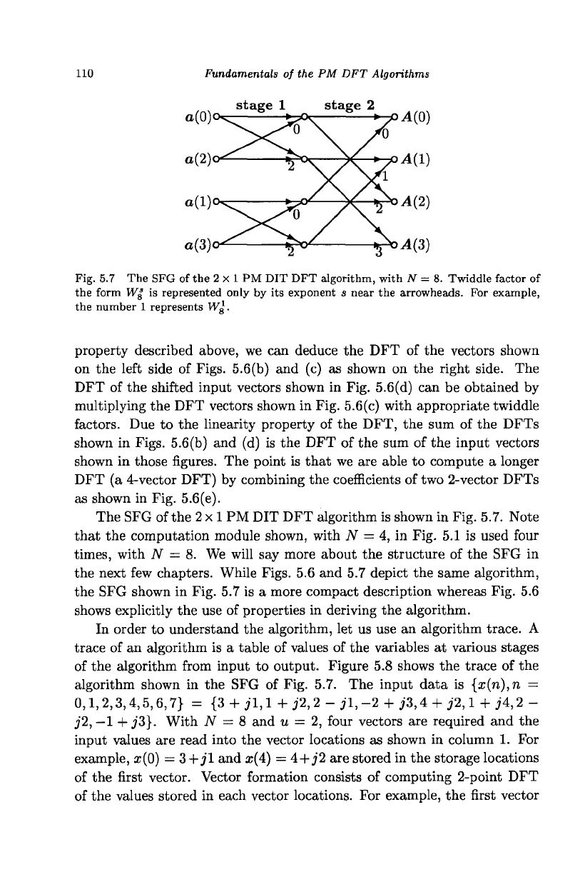
Fig. 5.8 The trace of the algorithm shown in Fig. 5.7.

is formed by adding and subtracting x(0) and x(4). In addition, vectors

are swapped to store them in a special order. More about this will be

said in the next chapter but, for the moment, remember that in Fig. 5.7

we have split the even and odd indexed input vectors into two groups.

After vector formation and swapping, we get the values shown in column 2.

Columns 3 and 4, respectively, show the values after the first and second

stage operations shown in SFG of Fig. 5.7 are carried out. Column 4 shows

the DFT values.

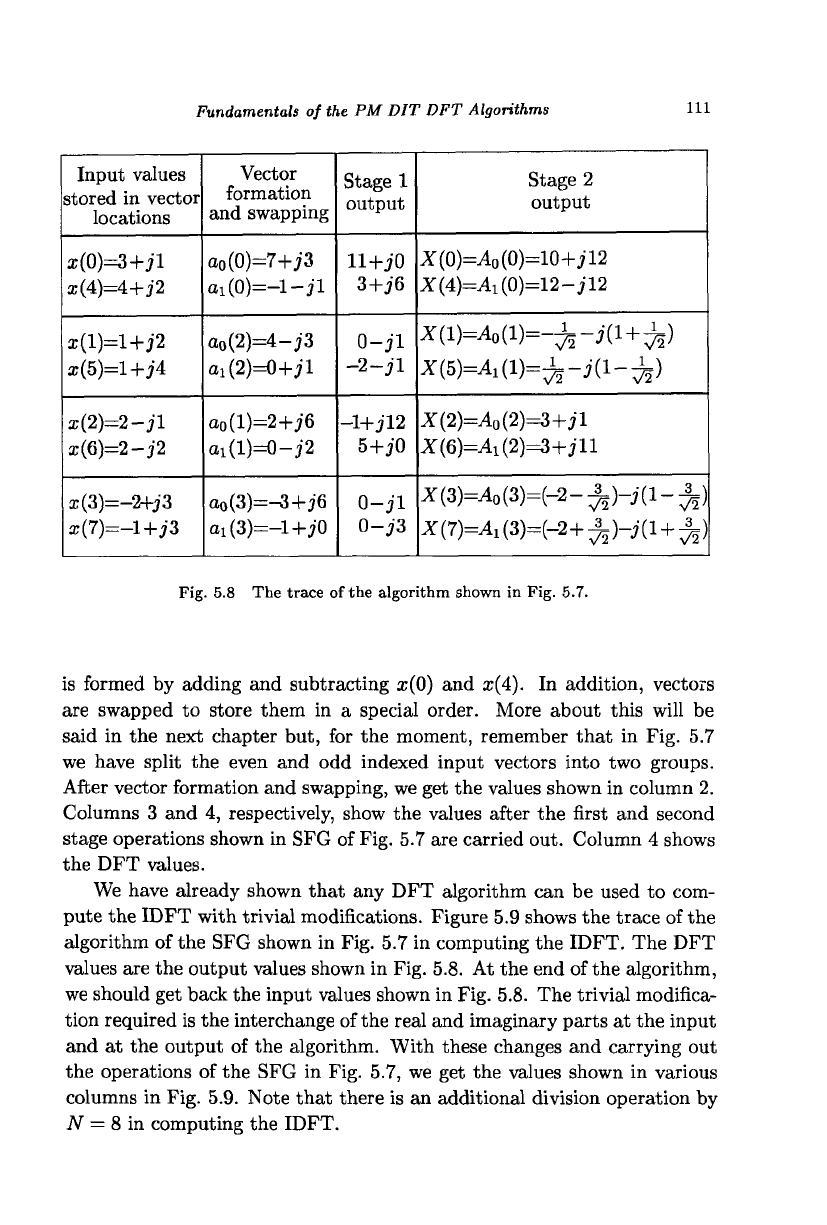
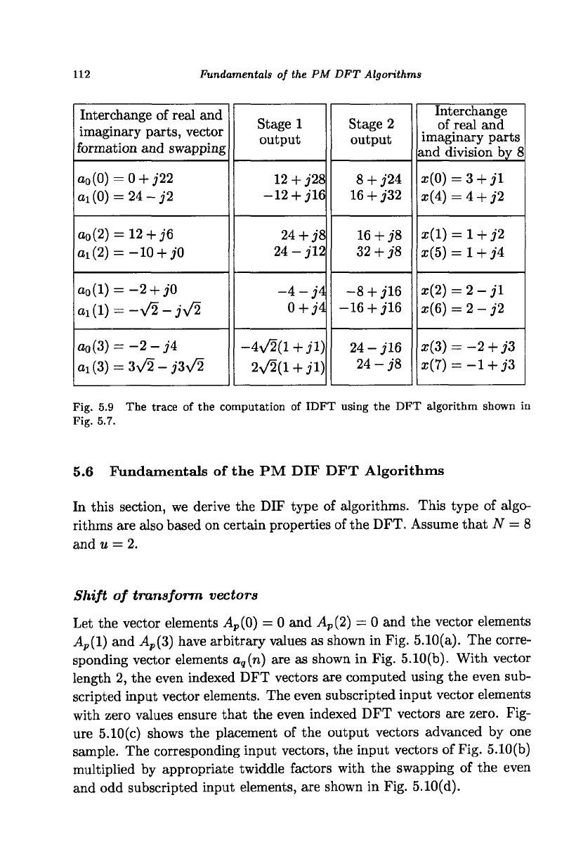
We have already shown that any DFT algorithm can be used to com-

pute the IDFT with trivial modifications. Figure 5.9 shows the trace of the

algorithm of the SFG shown in Fig. 5.7 in computing the IDFT. The DFT

values are the output values shown in Fig. 5.8. At the end of the algorithm,

we should get back the input values shown in Fig. 5.8. The trivial modifica-

tion required is the interchange of the real and imaginary parts at the input

and at the output of the algorithm. With these changes and carrying out

the operations of the SFG in Fig. 5.7, we get the values shown in various

columns in Fig. 5.9. Note that there is an additional division operation by

N = 8 in computing the IDFT.

112 Fundamentals of the PM DFT Algorithms

Interchange of real and

imaginary parts, vector

formation and swapping

(0)=0 + j22

ai(0) = 24-j2

(2) = 12+j6

ai(2) = -10 + j0

(l) = -2 + j0

Oi(l) = -\/2-jV2

(3) = -2-j4

Oi(3) = 3%/2-j3\/2

Stage 1

output

12 + j28

-12 + jW

24 + J8

24 - jl2

-4 - j4

0 + j4

-4v/2(l +jl)

2y/2(l + jl)

Stage 2

output

8 + j24

16 + j32

16 + J8

32 + j8

-8 + jl6

-16 + J16

24 - jl6

24 - j8

Interchange

of real and

imaginary parts

and division by 8

x(0)=3 + jl

x(4) = 4 + j2

x(l) = l+j2

x(5) = 1+ j4

x(2) = 2-jl

x(6) = 2 - j2

x(3) = -2 + j3

x(7) = -l + j3

Fig. 5.9 The trace of the computation of IDFT using the DFT algorithm shown in

Fig. 5.7.

5.6 Fundamentals of the PM DIF DFT Algorithms

In this section, we derive the DIF type of algorithms. This type of algo-

rithms are also based on certain properties of the DFT. Assume that N = 8

and u = 2.

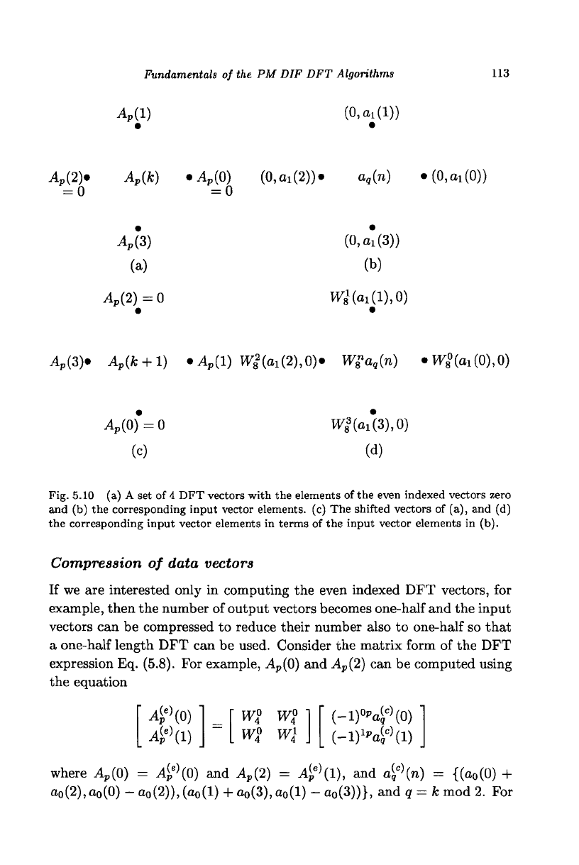
Shift of transform vectors

Let the vector elements A

(Q) = 0 and A

{2) = 0 and the vector elements

{\)

and A

(3) have arbitrary values as shown in Fig. 5.10(a). The corre-

sponding vector elements a

(n) are as shown in Fig. 5.10(b). With vector

length 2, the even indexed DFT vectors are computed using the even sub-

scripted input vector elements. The even subscripted input vector elements

with zero values ensure that the even indexed DFT vectors are zero. Fig-

ure 5.10(c) shows the placement of the output vectors advanced by one

sample. The corresponding input vectors, the input vectors of Fig. 5.10(b)

multiplied by appropriate twiddle factors with the swapping of the even

and odd subscripted input elements, are shown in Fig. 5.10(d).

Fundamentals of the PM DIF DFT Algorithms 113

(l)

(0,ai(l))

(2)*

(k) •ApiO) (0,ai(2)). a

(n) •(0,a

(0))

= 0

(3)

(a)

(2)

= 0

(0,a! (3))

(b)

W£(

(l),0)

4>(3)«

+1)

•^(1) W

(oi(2),0)« W£a

(n) • W

°(ai(0),0)

(0)

= 0

(c)

M3),0)

(d)

Fig. 5.10 (a) A set of

DFT vectors with the elements of the even indexed vectors zero

and (b) the corresponding input vector elements, (c) The shifted vectors of (a), and (d)

the corresponding input vector elements in terms of the input vector elements in (b).

Compression of data vectors

If we are interested only in computing the even indexed DFT vectors, for

example, then the number of output vectors becomes one-half and the input

vectors can be compressed to reduce their number also to one-half so that

a one-half length DFT can be used. Consider the matrix form of the DFT

expression Eq. (5.8). For example, A

(0) and A

(2) can be computed using

the equation

(o)

(e)

.rip

(l)

w? wl

(-1)°P4

(0)

(-i)^4

(i)

where A

{0) = A

(0) and A

(2) =

\l),

and a

\n) = {(o

(0) +

(2), a

(0) - a

(2)), (a

(l) + a

(3), a

(l) -

(3))},

and q = k mod 2. For