Sundararaja D. The Discrete Fourier Transform. Theory, Algorithms and Applications

Подождите немного. Документ загружается.

74 Properties of the DFT

storage locations are adequate to store an TV-point real-valued signal or its

spectrum.

Real signal with even symmetry

Since x(n)sin(^nfc) is an odd function of n, the imaginary part of the

DFT is zero. Therefore, as x(n) cos(^-nfc) is an even function of n, we get,

for JV even,

N-i

2?r

(k)

= X

—

k)='^2 x(n) cos -rj-nk

= z(0) + (-l)

x(y) + 2^x(n)cos^nfc

n=l

x(n) real and even

•&

X(k) real and even

Example 4.9

x(n) = {2,1,4,1} «- X(k) = {8, -2,4, -2}

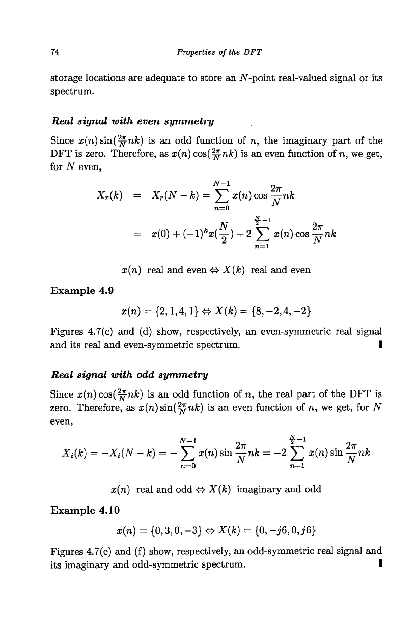
Figures 4.7(c) and (d) show, respectively, an even-symmetric real signal

and its real and even-symmetric spectrum. I

Real signal with odd symmetry

Since x(n) cos(^nfc) is an odd function of n, the real part of the DFT is

zero.

Therefore, as x(n)sm(^nk) is an even function of n, we get, for N

even,

Jv-i

f-i

2?r

Xi(k) = -Xi(N - k) = - ^ x(n) sin -rrnA; = -2 ^ x(n) sin -rjnk

n=0 n=l

x(n) real and odd

<S>

-XX&) imaginary and odd

Example 4.10

x{n) = {0,3,0, -3}

<£•

X(k) = {0, -j6,0, j6}

Figures 4.7(e) and (f) show, respectively, an odd-symmetric real signal and

its imaginary and odd-symmetric spectrum. I

Symmetry Properties

Real signal with even half-wave symmetry

The computation of the spectrum is equivalent to computing the DFT over

two periods of a periodic signal with period y. The DFT equation can be

written as

*(*) = £ ^

) +

(-!)**(»

J)WN (

-3)

n=0

Obviously, an even half-wave symmetric signal has odd-indexed DFT

coef-

ficients with zero value.

x(n) even half-wave symmetric

•&

X(k) even-indexed only and hermitian

Example 4.11

x(n) = {1,2,1,2} & X(k) = {6,0, -2,0}

Figures 4.7(g) and (h) show, respectively, an even half-wave symmetric real

signal and its hermitian-symmetric spectrum consisting of even-indexed

harmonics only. I

Real signal with odd half-wave symmetry

An odd half-wave symmetric signal has even-indexed DFT coefficients with

zero value, which is evident from Eq. (4.3).

x(n) odd half-wave symmetric

X(k) odd-indexed only and hermitian

Example 4.12

x(n) - {1,2, -1, -2} &X(k) = {0,2 - j'4,0,2 + j4}

Figures 4.7(i) and (j) show, respectively, an odd half-wave symmetric real

signal and its hermitian-symmetric spectrum consisting of odd-indexed har-

monics only. I

Imaginary signal

This case is similar to that of the real-valued signal except that the data

values are multiplied by the complex constant

Therefore,

(k)

= -X

(N - k) and X^k) = X

(N - k)

76 Properties of the DFT

x(n) imaginary & X(k) antihermitian

Example 4.13

x(n) = {J2,jl,j4,j3} &X(k) = {jlO, -2 - j2, j2,2 - j2}

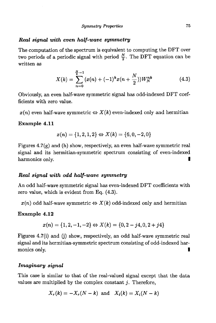
Figures 4.8(a) and (b) show, respectively, an imaginary signal and its anti-

hermitian spectrum. I

Imaginary signal with even symmetry

x(n) imaginary and even O^ X(k) imaginary and even

Example 4.14

x(n) = {J2,jl,j4,jl} & X(k) = {j8, -J2J4, -j2}

Figures 4.8(c) and (d) show, respectively, an imaginary signal with even

symmetry and its imaginary and even-symmetric spectrum. I

Imaginary signal with odd symmetry

x(n) imaginary and odd

•£>

X(k) real and odd

Example 4.15

x{n) =

{0,

j3,0, -j3} & X(k) = {0,6,0, -6}

Figures 4.8(e) and (f) show, respectively, an imaginary signal with odd

symmetry and its real and odd-symmetric spectrum. I

Imaginary signal with even half-wave symmetry

x(n)even half-wave symmetric<^-X(fe)even-indexed only and antihermitian

Example 4.16

z(n) = {jl,j2,jl,j2}&X{k) = {j6,0,-j2,0}

Symmetry Properties

o^X^^

(a)

(i)

10 15

3? 4

-4

•real

o imaginary

5 10

(b)

5 °

o •

-4 ,

5 10 15

(d)

jX. op» o • o

5 10

-4(<

£ Oh. •

5 10 15

-4

• :

(h)

o o

. •

5 10

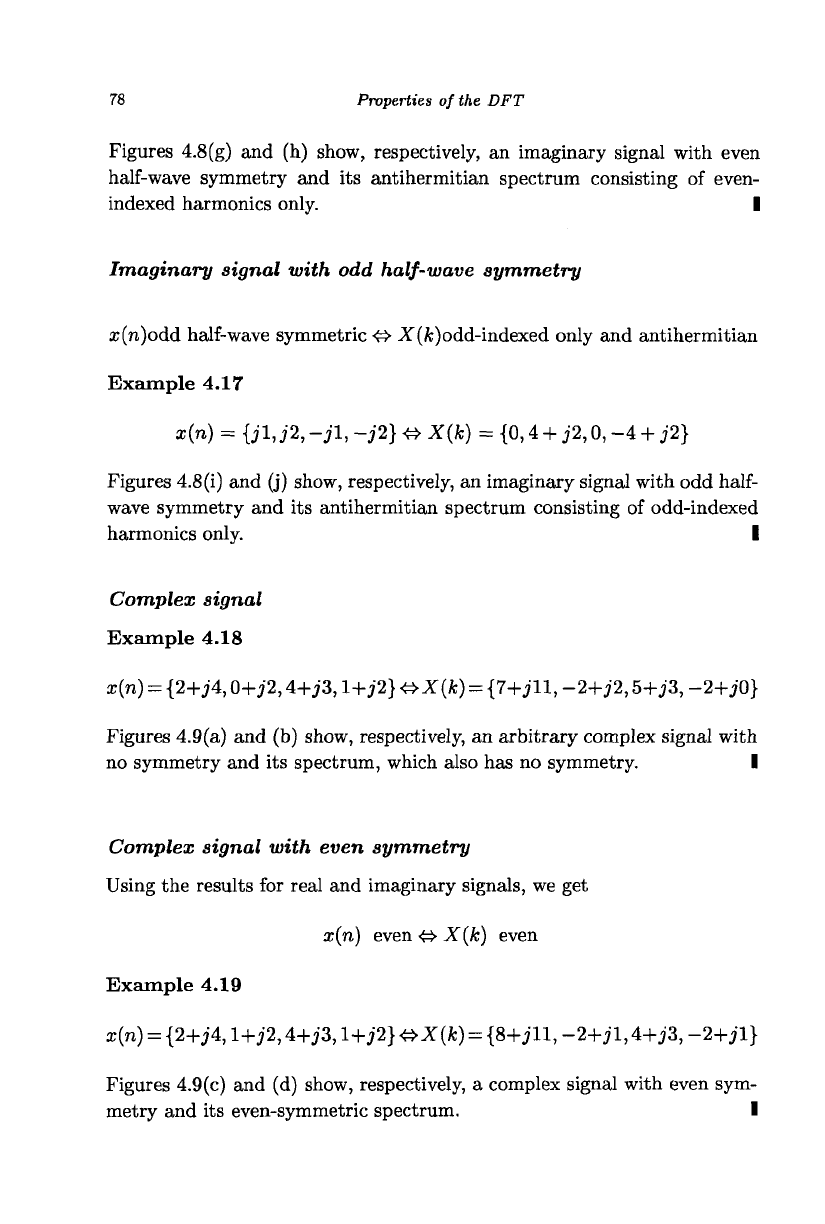
Fig. 4.8 (a) An imaginary signal and (b) its antihermitian-symmetric spectrum, (c) An

even-symmetric imaginary signal and (d) its imaginary and even-symmetric spectrum.

(e) An odd-symmetric imaginary signal and (f) its real and odd-symmetric spectrum.

(g) An imaginary signal with even half-wave symmetry and (h) its spectrum with even-

indexed harmonics only, (i) An imaginary signal with odd half-wave symmetry and (j)

its spectrum with odd-indexed harmonics only.

Properties of the DFT

Figures 4.8(g) and (h) show, respectively, an imaginary signal with even

half-wave symmetry and its antihermitian spectrum consisting of even-

indexed harmonics only. I

Imaginary signal with odd half-wave symmetry

x(n)odd half-wave symmetric

<4-

X(fc)odd-indexed only and antihermitian

Example 4.17

x(n) = {jl,j2, -jl, -j2} & X(k) = {0,4 + j2,0, -4 + j2}

Figures 4.8(i) and (j) show, respectively, an imaginary signal with odd

half-

wave symmetry and its antihermitian spectrum consisting of odd-indexed

harmonics only. I

Complex signal

Example 4.18

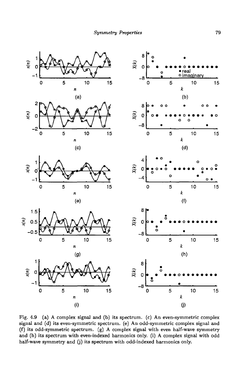
x{n) = {2+J4,0+j2,4+j3,1+j2} &X(k) = {7+jll, -2+J2,5+J3, -2+jO}

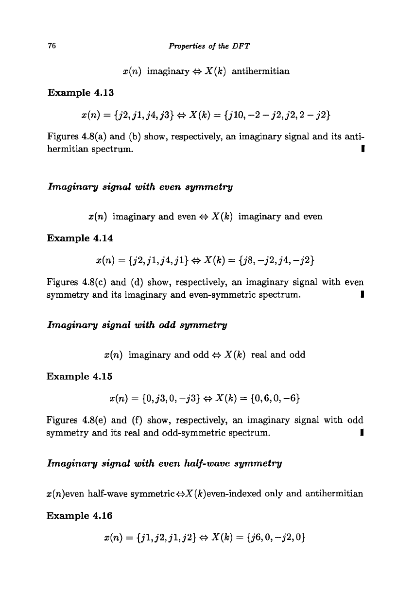
Figures 4.9(a) and (b) show, respectively, an arbitrary complex signal with

no symmetry and its spectrum, which also has no symmetry. I

Complex signal with even symmetry

Using the results for real and imaginary signals, we get

x(n) even &X (k) even

Example 4.19

x{n) = {2+jA, 1+J2,4+J3,1+J2} &X{k) = {8+jll, -2+jl,

4+J3,

-2+jl}

Figures 4.9(c) and (d) show, respectively, a complex signal with even sym-

metry and its even-symmetric spectrum. I

Symmetry Properties

_^ 1

"Br

-1

I o

vlj

"*r o'

-1

/>/

'\7

1.5

5 0.5

-0.5

y v

"? n

a/30? /

\ ^

J'V

^yw

(a)

a f*

A./ /

^\^y

(c)

,^l

r \

!)dt

y>Af

(g)

\j£^m\

V w\j

(

^/V

A£

J? 0

•

o •

-8

o a

•

o •

1 °

-4

•

• • 0

-8

•

$< 0

-8

• •

•

O O

a O

•

• real

o imaqinarv

(b)

• o o

o o

•

(d)

• • • • o •

•

(h)

•

O a

10 15 10 15

(J)

Fig. 4.9 (a) A complex signal and (b) its spectrum, (c) An even-symmetric complex

signal and (d) its even-symmetric spectrum, (e) An odd-symmetric complex signal and

(f) its odd-symmetric spectrum, (g) A complex signal with even half-wave symmetry

and (h) its spectrum with even-indexed harmonics only, (i) A complex signal with odd

half-wave symmetry and (j) its spectrum with odd-indexed harmonics only.

Properties

of the DFT

Complex signal with

odd

symmetry

x(n)

odd O X(fc) odd

Example

4.20

x(n)

{0,1

j2,0,

-1 -

j2}

&X{k) = {0,4 -

j2,0,

-4 + j2}

Figures 4.9(e)

and (f)

show, respectively,

complex signal with

odd

sym-

metry

and its

odd-symmetric spectrum.

Complex signal with even half-wave symmetry

x(n) even half-wave symmetric

O X(k)

even-indexed only

Example

4.21

x(n)

= {2 + j3,1 - jl,2 +

j3,1

- jl}

<S>

X(k) = {6 +

j4,0,2

+ j8,0}

Figures 4.9(g)

and (h)

show, respectively,

complex signal with even

half-

wave symmetry

and its

spectrum consisting

even-indexed harmonics only.

Complex signal with

odd

half-wave symmetry

x(n)

odd

half-wave symmetric

O- X

(k) odd-indexed only

Example

4.22

x(n)

+ jl,

j2,

-1 - jl, -2 - j2} & X(k) = {0,6 - j2,0, -2 + j6}

Figures 4.9(i)

and (j)

show, respectively,

complex signal with

odd half-

wave symmetry

and its

spectrum consisting

odd-indexed harmonics only.l

Representation

of a

signal defined over

finite range

DFT

analysis,

it is

assumed that

the

signal

periodic.

the objective

to represent

the

signal only over

the

defined finite range, then

the

function

can

arbitrarily extended

and the

denned range along with

the

extension

can

considered

as the

fundamental period

of the

signal.

The

extension

Transform of Complex Conjugates

* 0

(a)

X OP o (

-. 16

•

real .

imaginary

5 10

(b)

•0

10 20

(c)

(d)

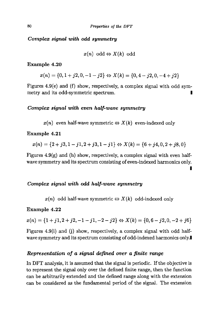
Fig. 4.10 (a) A real signal and (b) its spectrum with several nonzero coefficients, (c) The

extension of the signal shown in (a), and (d) its spectrum with only a pair of nonzero

coefficients.

of the signal can be made in several ways and the DFT representation of

all of them will represent the signal correctly in the defined range.

Given the freedom to arbitrarily extend the signal, it is desirable to ex-

tend so that the signal is adequately represented by as few coefncients as

possible. The basic consideration is to extend the signal so that the exten-

sion does not create any discontinuities. The more smoother the extension

the smaller is the set of coefficients required to represent the signal.

Example 4.23 Figures 4.10 (a) and (b) show, respectively, half period

of a sine waveform and its spectrum. In this representation, the half period

waveform is considered as the fundamental period. If we extend the signal

as shown in Fig. 4.10(c) and compute the DFT, we get the spectrum shown

in Fig. 4.10(d). The difference between the spectra is that the first spectrum

has several nonzero frequency coefficients whereas the second spectrum has

only two and is, obviously, a more efficient representation. I

4.7 Transform of Complex Conjugates

The conjugation operation reflects the vector represented by a complex

number about the real axis, that is the imaginary part is negated. Let

x(n) &X(k). Then,

x*(n)&X*(N -k) and x*(N - n)

X*(k)

Properties of the DFT

Conjugating both sides of Eq. (3.6), we get

JV-l JV-l

X*(k)

= Y,

x*{n)W^

= J2 **(

n)W^

n=0 n=0

Conjugating both sides of Eq. (3.6) and substituting k = N

—

k, we get

JV-l

X*(N-k)=J2x*(n)W%

, k =

0,l,...N-l

71=0

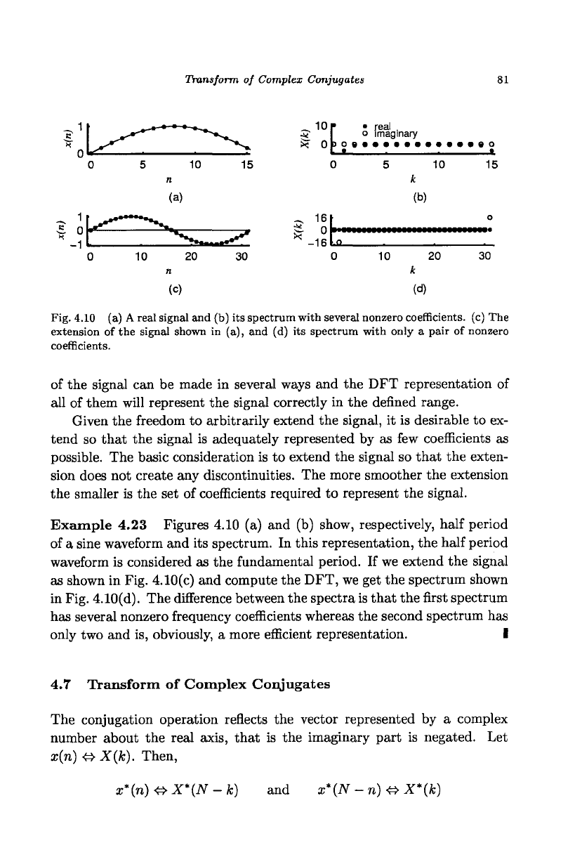
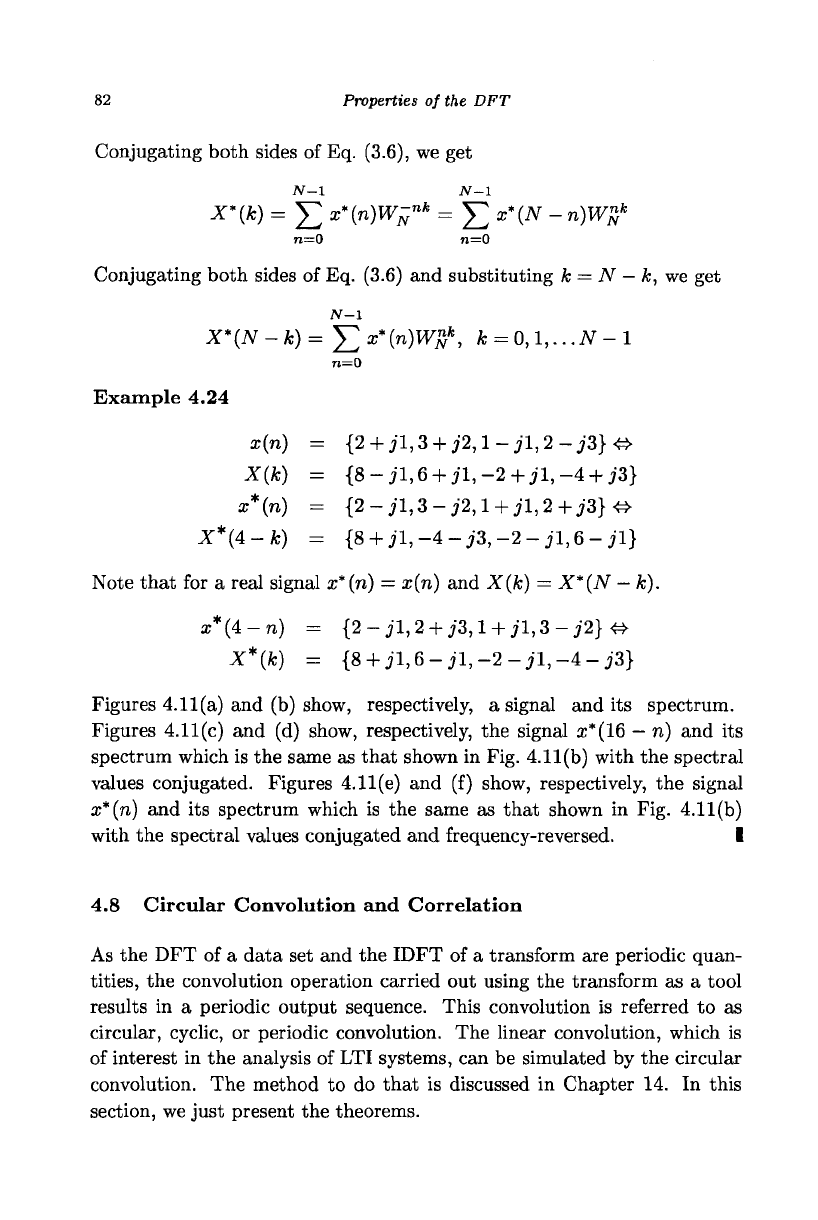
Example 4.24

x{n) = {2 + jl,3 + j2,l-jl,2-j3}&

X(k) = {8 - jl, 6 + il, -2 + jl, -4 + j3}

x*(n) = {2-jl,Z-j2,l + jl,2+j3}&

X*(4-k)

= {

+ jl,-4-A-2-jl,6-jl}

Note that for a real signal x*(n) = x{n) and X{k) = X*(N

—

k).

ar*(4-n) = {2 - jl,2 + j3,l + jl,3 - j2} &

X*(k)

= {8

jl,6-jl,-2-jl,-A-j3}

Figures 4.11(a) and (b) show, respectively, a signal and its spectrum.

Figures 4.11(c) and (d) show, respectively, the signal x*(16 - n) and its

spectrum which is the same as that shown in Fig. 4.11(b) with the spectral

values conjugated. Figures 4.11(e) and (f) show, respectively, the signal

x*(n)

and its spectrum which is the same as that shown in Fig. 4.11(b)

with the spectral values conjugated and frequency-reversed. I

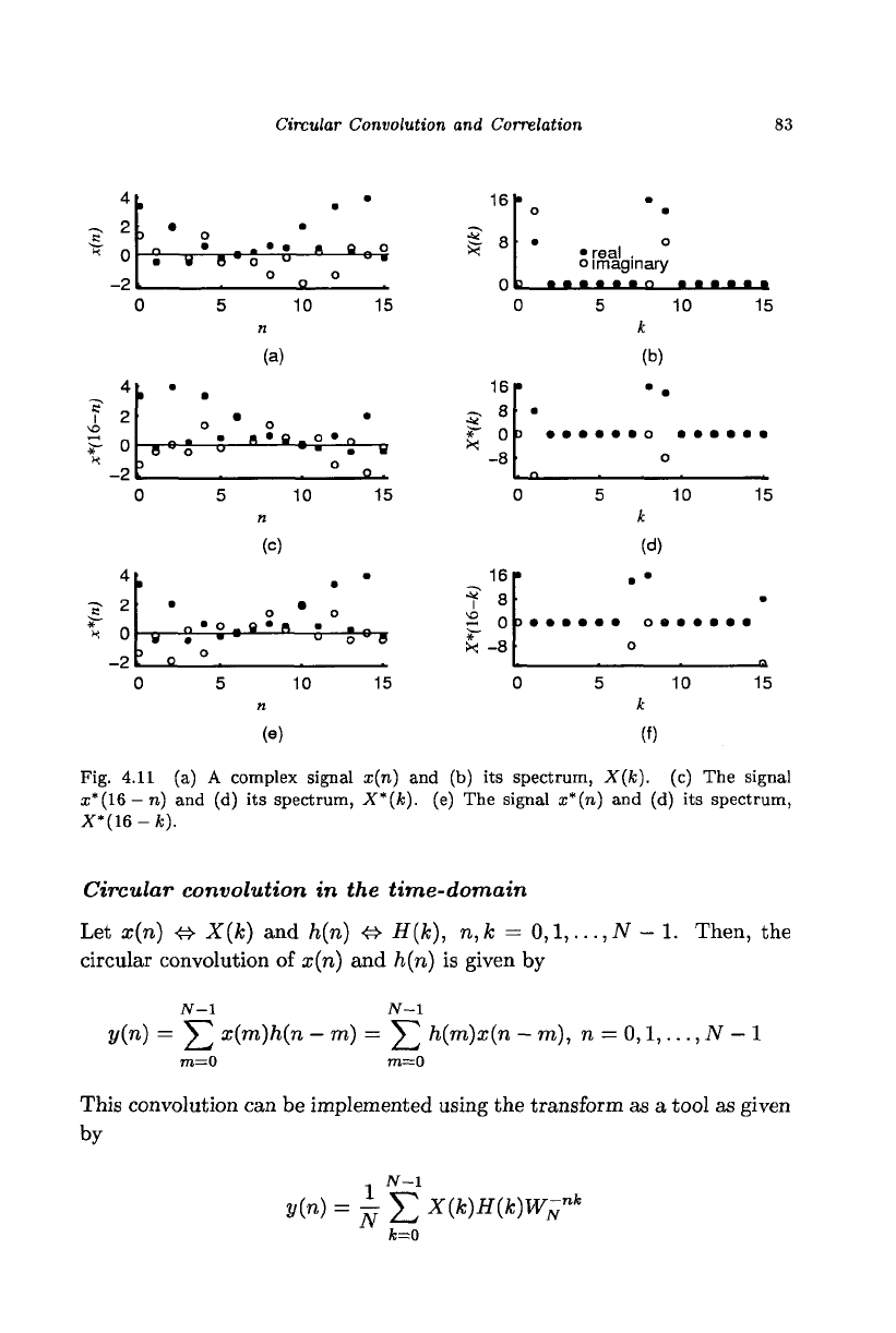
4.8 Circular Convolution and Correlation

As the DFT of a data set and the IDFT of a transform are periodic quan-

tities,

the convolution operation carried out using the transform as a tool

results in a periodic output sequence. This convolution is referred to as

circular, cyclic, or periodic convolution. The linear convolution, which is

of interest in the analysis of LTI systems, can be simulated by the circular

convolution. The method to do that is discussed in Chapter 14. In this

section, we just present the theorems.

Circular Convolution and Correlation 83

n * _ * • A Q O

u B'5 " "

°»

-2C

T*o

5 10

(a)

"'»•;'"

-2

5 10 15

(c)

S'S'

' 5°a

5 10

(•)

• real .

o imaginary

»«»»»•"

• t t t • •

0 5 10

(b)

*~ Qp •••••• o ••••

-8

5 10

(d)

-8

•

)••••••

O B • • • • •

-_ . . a

5 10

Fig. 4.11 (a) A complex signal x(n) and (b) its spectrum, X(k). (c) The signal

i*(16 —n) and (d) its spectrum,

X"(k).

(e) The signal x*(n) and (d) its spectrum,

X*(16-ifc).

Circular convolution in the time-domain

Let x{n) 4> X{k) and h(n) 4> H(k), n,k =

0,1,..., JV

- 1. Then, the

circular convolution of x(n) and h(n) is given by

JV-l JV-1

y(n) = Y^ x(m)h(n

—

rn) = Y^ /i(m)a;(n - m), n =

0,1,...,

—

m=0 m=0

This convolution can be implemented using the transform as a tool as given

7V-1

»(»)

^ E

*(*)#

(*w*

fc=0