Simon Benninga. Financial Modelling 3-rd edition

Подождите немного. Документ загружается.

278 Chapter 9

9.7 Finding the Market Portfolio: The Capital Market Line

Suppose a risk-free asset exists, and suppose that this asset has expected

return r

. Let M be the efﬁ cient portfolio that is the solution to the system

of equations

Er r Sz

()−=

∑

Now consider a convex combination of the portfolio M and the risk-free

asset r

; for example, suppose that the weight of the risk-free asset in such

a portfolio is a. It follows from the standard equations for portfolio

return and s that

E r ar a E r

aaaarr

pf M

pr M fy

() ( )( )

() ()()

=+−

=+−+− =

121

22 22

σσ σ

Cov , (()1−a

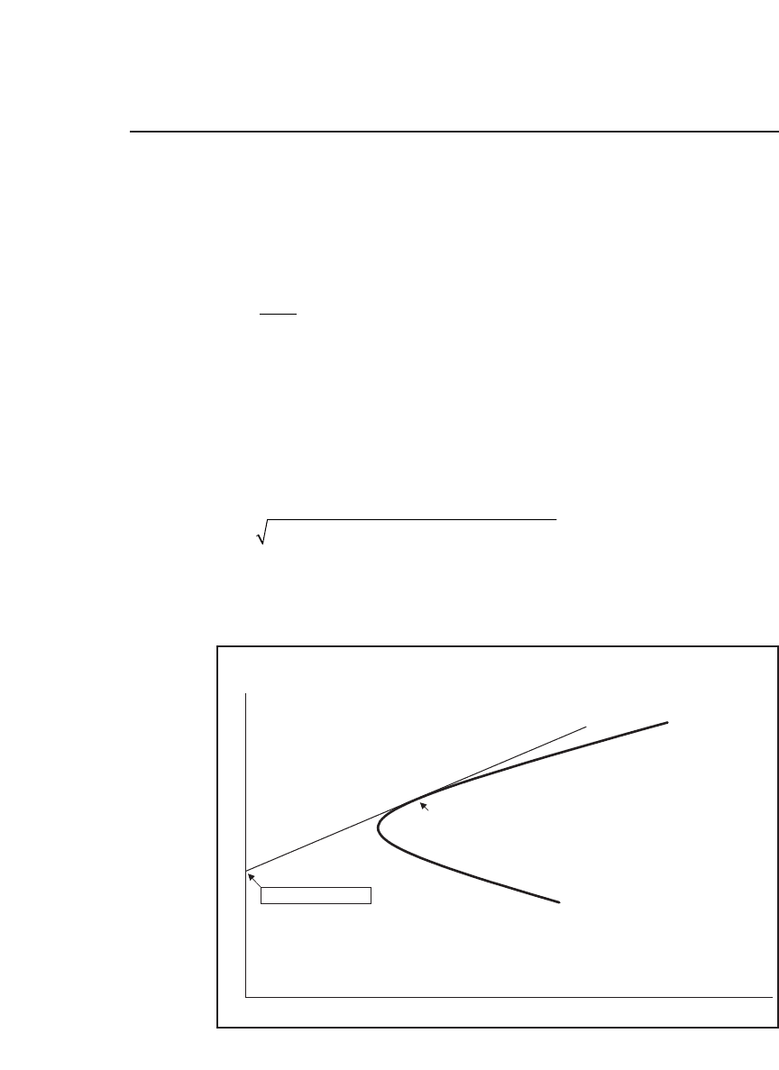
The locus of all such combinations for a ≥ 0 is known as the capital market

line (CML). It appears along with the efﬁ cient frontier in the following

graph:

Efficient Frontier with CML

Portfolio standard deviation

Portfolio mean return

Market

portfolio, M

Capital market line, CML

Risk-free rate, r

279 Calculating Efﬁ cient Portfolios When There Are No Short-Sale Restrictions

The portfolio M is called the market portfolio for several reasons:

•

Suppose investors agree about the statistical portfolio information [i.e.,

the vector of expected returns E(r) and the variance-covariance matrix

S]. Suppose furthermore that investors are interested only in maximizing

expected portfolio return given portfolio standard deviation s. Then it

follows that all optimal portfolios will lie on the CML.

•

In this case, it further follows that the portfolio M is the only portfolio

of risky assets included in any optimal portfolio. Portfolio M must there-

fore include all the risky assets, with each asset weighted in proportion to

its market value. That is,

Weight of risky asset in portfolioiM

∑

where V

is the market value of asset i.

It is not difﬁ cult to ﬁ nd M when we know r

: We merely have to solve for

the efﬁ cient portfolio given that the constant c = r

. When r

changes, we get

a different “market” portfolio—this is just the efﬁ cient portfolio given a

constant of r

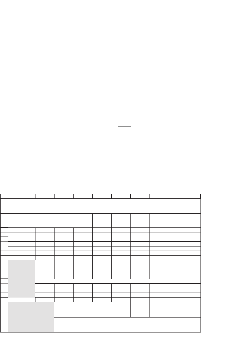
. For example, in our numerical example, suppose that the

risk-free rate is r

= 5 percent. Then solving the system E(r) − r

= Sz gives

ABCDEFG H

Expected

returns

E(r)

0.40 0.03 0.02 0.00 0.06

0.03 0.20 0.00 -0.06 0.05

0.02 0.00 0.30 0.03 0.07

0.00 -0.06 0.03 0.10 0.08

Constant 0.05

Envelope

portfolio

is market

portfolio M

0.0314 <-- {=MMULT(MINVERSE(A3:D6),F3:F6-B8)/SUM(MMULT(MINVERSE(A3:D6),F3:F6-B8))}

0.2059

0.0597

0.7031

Portfolio

expected

return, E(r

)

7.26% <-- =SUMPRODUCT(A11:A14,F3:F6)

Portfolio

standard

devation,

21.21% <-- {=SQRT(MMULT(MMULT(TRANSPOSE(A11:A14),A3:D6),A11:A14))}

WHEN c = r

THE ENVELOPE PORTFOLIO

IS THE MARKET PORTFOLIO M

Variance-covariance matrix

280 Chapter 9

9.8 Testing the SML: Implementing Propositions 3–5

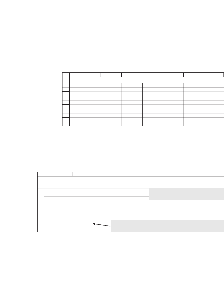
To illustrate Propositions 3–5, consider the following data for four risky

assets:

ABCDE F

Dates Asset 1

Asset 2 Asset 3 Asset 4

1 -6.63% -2.49% -4.27% 11.72%

2 8.53% 2.44% -3.15% -8.33%

3 1.79% 4.46% 1.92% 19.18%

4 7.25% 17.90% -6.53% -7.41%

5 0.75% -8.22% -1.76% -1.44%

6 -1.57% 0.83% 12.88% -5.92%

7 -2.10% 5.14% 13.41% -0.46%

Mean 1.15% 2.87% 1.79% 1.05% <-- =AVERAGE(E3:E9)

ILLUSTRATING PROPOSITIONS 3-5

The asset returns on seven dates are given in rows 3–9, and the average

return is given in row 11.

We use some sophisticated array functions to compute the variance-

covariance matrix:

GFEDCBA

Variance-covariance matrix

Asset 1 Asset 2 Asset 3 Asset 4

Asset 1 0.0024 0.0019 -0.0015 -0.0024

Asset 2 0.0019 0.0056 -0.0007 -0.0016

Asset 3 -0.0015 -0.0007 0.0057 -0.0005

Asset 4 -0.0024 -0.0016 -0.0005 0.0094

Finding an efficient portfolio w

Constant 0.50%

Asset 1 0.3129

Asset 2 0.2464

Asset 3 0.2690

Asset 4 0.1717

Cells B23:B26 contain the formula

{=MMULT(MINVERSE(B15:E18),TRANSPOSE(B11:E11)-

B21)/SUM(MMULT(MINVERSE(B15:E18),TRANSPOSE(B11:E11)-B21))}

cells B15:E18 contain the formula

{=MMULT(TRANSPOSE(B3:E9-B11:E11),B3:E9-

B11:E11)/7}

The efﬁ cient portfolio given the constant c = 0.5 percent is given in

cells B23 : B26; we compute this portfolio using the method of Proposi-

tion 1.

We call this portfolio w. The returns of portfolio w on dates 1–7

are given in column G, as follows.

3. Following the discussion in section 9.5, a careful reader will recall that Proposition 1

only guarantees that this portfolio is on the envelope. But it is, in fact, efﬁ cient.

281 Calculating Efﬁ cient Portfolios When There Are No Short-Sale Restrictions

We illustrate Propositions 3–5 in two steps:

•

Step 1: We regress the returns of each asset on the returns of the efﬁ -

cient portfolio: For i = 1, . . . , 4 we run the regression r

= a

+ b

+ e

This regression is often called the ﬁ rst-pass regression. The results are as

follows:

GFEDCBA H

Dates Asset 1 Asset 2 Asset 3

Asset 4 Efficient portfolio w

1 -6.63% -2.49% -4.27% 11.72% -1.82% <-- {=MMULT(B3:E9,B23:B26)}

2 8.53% 2.44% -3.15% -8.33% 0.99%

3 1.79% 4.46% 1.92% 19.18% 5.47%

4 7.25% 17.90% -6.53% -7.41% 3.65%

5 0.75% -8.22% -1.76% -1.44% -2.51%

6 -1.57% 0.83% 12.88% -5.92% 2.16%

7 -2.10% 5.14% 13.41% -0.46% 4.14%

Mean 1.15% 2.87% 1.79% 1.05% <-- =AVERAGE(E3:E9) 1.73%

FEDCBA

Implementing propositions 3-5--finding the SML

Step 1: Regress each asset's returns on those of the efficient portfolio w

Asset 1 Asset 2 Asset 3 Asset 4

Alpha 0.0024 -0.0047 -0.0002 0.0028 <-- =INTERCEPT(E3:E9,$G$3:$G$9)

Beta 0.5284 1.9301 1.0490 0.4478 <-- =SLOPE(E3:E9,$G$3:$G$9)

R-squared 0.0897 0.5241 0.1505 0.0167 <-- =RSQ(E3:E9,$G$3:$G$9)

•

Step 2: We now regress the betas of the assets on their mean returns.

Running this regression, r¯

= g

+ g

+ e

, gives

ABCD

Step 2: Regress the asset mean returns on their betas

Intercept 0.005 <-- =INTERCEPT(B11:E11,B33:E33)

Slope 0.0123 <-- =SLOPE(B11:E11,B33:E33)

R-squared 1.0000 <-- =RSQ(B11:E11,B33:E33)

To check the results of Propositions 3–5, we run a test:

ABCD

Intercept = c ? yes <-- =IF(B36=B20,"yes","no")

Slope = E(r

) - c ?

yes <-- =IF(B38=G11-B21,"yes","no")

Check Propositions 3 & 4: Step-2 coefficients should be

Intercept = c, Slope = E(r

) - c

The “perfect” regression results (note the R

= 1 in cell B39) are the

results promised us by Propositions 3–5:

282 Chapter 9

•

The second-pass regression intercept is equal to c, and the slope is

equal to E(r

) − c.

•

If there is a riskless asset with return c = r

, then Proposition 5 prom-

ises that in the second-pass regression r¯

= g

+ g

+ e

, g

= r

, and

= E(r

) − r

•

If there is no riskless asset, then Proposition 3 states that in the second-

pass regression g

= E(r

) and g

= E(r

) − E(r

), where z is a portfolio

whose covariance with w is zero.

•

Finally, if we run a two-stage regression of the type described on any

portfolio w and get a “perfect regression,” then Proposition 4 guarantees

that w is in fact efﬁ cient.

To drive home the point that this technique always works, we show

you all the calculations using a different value for c (cell B21, highlighted

in the following spreadsheet). As proved in Propositions 3–5, the result

is still a perfect regression of the means on the betas.

GFEDCBA H

Dates Asset 1 Asset 2 Asset 3 Asset 4

Efficient portfolio w

1 -6.63% -2.49% -4.27% 11.72% -2.95% <-- {=MMULT(B3:E9,B23:B26)}

2 8.53% 2.44% -3.15% -8.33% 3.64%

3 1.79% 4.46% 1.92% 19.18% 5.16%

4 7.25% 17.90% -6.53% -7.41% -2.40%

5 0.75% -8.22% -1.76% -1.44% 2.24%

6 -1.57% 0.83% 12.88% -5.92% 0.01%

7 -2.10% 5.14% 13.41% -0.46% -0.26%

Mean 1.15% 2.87% 1.79% 1.05% <-- =AVERAGE(E3:E9) 0.78%

Variance-covariance matrix

Asset 1 Asset 2 Asset 3 Asset 4

Asset 1 0.0024 0.0019 -0.0015 -0.0024 <-- {=MMULT(TRANSPOSE(B3:E9-B11:E11),B3:E9-B11:E11)/7}

Asset 2 0.0019 0.0056 -0.0007 -0.0016

Asset 3 -0.0015 -0.0007 0.0057 -0.0005

Asset 4 -0.0024 -0.0016 -0.0005 0.0094

Finding an efficient portfolio w

Constant 2.00%

Asset 1 0.8234 <-- {=MMULT(MINVERSE(B15:E18),TRANSPOSE(B11:E11)-B21)/SUM(MMULT(MINVERSE(B15:E18),TRANSPOSE(B11:E11)-B21))}

Asset 2 -0.2869

Asset 3 0.2278

Asset 4 0.2357

Implementing propositions 3-5--finding the SML

Step 1: Regress each asset's returns on those of the efficient portfolio w

Asset 1 Asset 2 Asset 3 Asset 4

Alpha 0.0061 0.0342 0.0165 0.0044 <-- =INTERCEPT(E3:E9,$G$3:$G$9)

Beta 0.6968 -0.7075 0.1752 0.7776 <-- =SLOPE(E3:E9,$G$3:$G$9)

R-squared 0.1570 0.0709 0.0042 0.0506 <-- =RSQ(E3:E9,$G$3:$G$9)

Step 2: Regress the asset mean returns on their betas

Intercept 0.02 <-- =INTERCEPT(B11:E11,B33:E33)

Slope -0.0122 <-- =SLOPE(B11:E11,B33:E33)

R-squared 1.0000 <-- =RSQ(B11:E11,B33:E33)

Intercept = c ? yes <-- =IF(B36=B20,"yes","no")

Slope = E(r

) - c ?

yes <-- =IF(B38=G11-B21,"yes","no")

Check Propositions 3 & 4: Step 2 coefficients should be:

Intercept = c, Slope = E(r

) - c

ILLUSTRATING PROPOSITIONS 3-5

This time the constant is 2% (cell B21)

283 Calculating Efﬁ cient Portfolios When There Are No Short-Sale Restrictions

9.9 Summary

In this chapter we have presented theorems relating to efﬁ cient portfo-

lios and then showed how to implement these theorems to ﬁ nd the efﬁ -

cient frontier. Two basic propositions allow us to derive portfolios on the

envelope of the feasible set of portfolios and the envelope itself. Three

further propositions relate the expected returns of any asset or portfolio

to the expected returns on any efﬁ cient portfolio. Under certain circum-

stances, these propositions allow us to derive the security market line

(SML) and the capital market line (CML) of the classic capital asset

pricing model (CAPM).

In subsequent chapters we discuss the implementation of the CAPM.

We show how to compute the variance-covariance matrix (Chapter 10),

how to test the SML (Chapter 11), how to optimize in the presence of

short-sale constraints (Chapter 12), and how to derive useful portfolio

optimization routines from our knowledge of efﬁ cient set mathematics

(Chapter 13, which discusses the Black-Litterman model).

Exercises

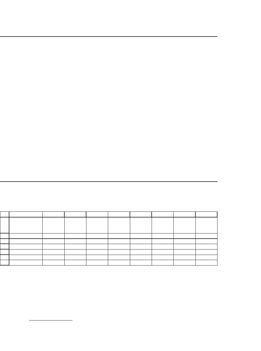
1. Consider the following data for six furniture companies:

ABCDEFGH

Variance-

covariance

matrix

La-Z-Boy Kimball Flexsteel Leggett Miller Shaw Means

La-Z-Boy

0.1152 0.0398 0.1792 0.0492 0.0568 0.0989 29.24%

Kimball

0.0398 0.0649 0.0447 0.0062 0.0349 0.0269 20.68%

Flexsteel

0.1792 0.0447 0.3334 0.0775 0.0886 0.1487 25.02%

Leggett

0.0492 0.0062 0.0775 0.1033 0.0191 0.0597 31.64%

Mille

0.0568 0.0349 0.0886 0.0191 0.0594 0.0243 15.34%

Shaw

0.0989 0.0269 0.1487 0.0597 0.0243 0.1653 43.87%

a. Given this matrix, and assuming that the risk-free rate is 0 percent, calculate the

efﬁ cient portfolio of these six ﬁ rms.

b. Repeat, assuming that the risk-free rate is 10 percent.

c. Use these two portfolios to generate an efﬁ cient frontier for the six furniture

companies. Plot this frontier.

d. Is there an efﬁ cient portfolio with only positive proportions of all the assets?

4. The problem of when a portfolio contains only positive weights in nontrivial. See the

articles by Green (1986) and Nielsen (1987).

284 Chapter 9

2. A sufﬁ cient condition to produce positively weighted efﬁ cient portfolios is that the

variance-covariance matrix be diagonal: That is, that s

= 0, for i ≠ j. By continuity,

positively weighted portfolios will result if the off-diagonal elements of the

variance-covariance matrix are sufﬁ ciently small compared to the diagonal. Con-

sider a transformation of the preceding matrix in which

εσ

ij=

⎧

⎨

⎩

≠

Original

When ε = 1, this transformation will give the original variance-covariance matrix,

and when ε = 0, the transformation will give a fully diagonal matrix.

For r = 10 percent, ﬁ nd the maximum ε for which all portfolio weights are

positive.

3. In the following example, use Excel to ﬁ nd an envelope portfolio whose b with

respect to the efﬁ cient portfolio y is zero. Hint: Notice that because the covariance

is linear, so is b: Suppose that z = lx + (1 − l)y is a convex combination of x and y,

and that we are trying to ﬁ nd the b

. Then

λλ

zy x yy

xy y

+−

−

Cov( , ) Cov[ , ]

Cov( , ) Cov(

()

,, )y

λβ λ

1=+−()

ABCDEF

Mean

returns

0.400 0.030 0.020 0.000 0.06

0.030 0.200 0.001 -0.060 0.05

0.020 0.001 0.300 0.030 0.07

0.000 -0.060 0.030 0.100 0.08

Variance-covariance matrix

4. Calculate the envelope set for the following four assets and show that the individual

assets all lie within this envelope set.

ABCDEF

Mean returns

0.10 0.01 0.03 0.05 6%

0.01 0.30 0.06 -0.04 8%

0.03 0.06 0.40 0.02 10%

0.05 -0.04 0.02 0.50 15%

A FOUR-ASSET PORTFOLIO PROBLEM

Variance-covariance

285 Calculating Efﬁ cient Portfolios When There Are No Short-Sale Restrictions

Appendix

In this appendix we collect the various proofs of statements made in the

chapter. As in the chapter, we assume that we are examining data for N

risky assets. It is important to note that all the deﬁ nitions of “feasibility”

and “optimality” are made relative to this set. Thus the phrase “efﬁ cient”

really means “efﬁ cient relative to the set of the N assets being

examined.”

proposition 0 The set of all feasible portfolios of risky assets is

convex.

Proof A portfolio x is feasible if and only if the proportions of the

portfolio add up to 1; that is, x

∑

where N is the number of risky

assets. Suppose that x and y are feasible portfolios and suppose that l is

some number between 0 and 1. Then it is clear that z = lx + (1 − l)y is

also feasible.

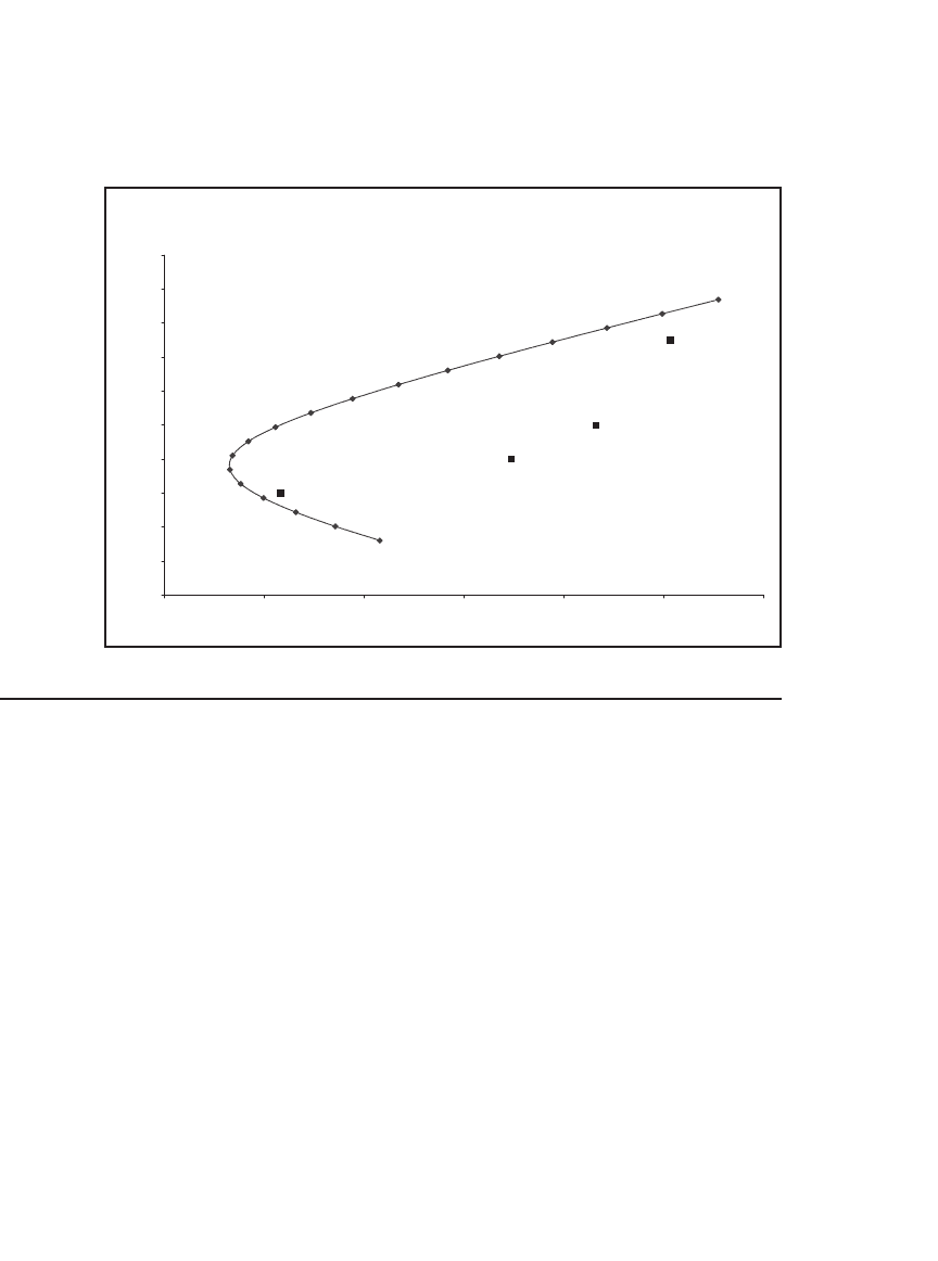
You should get a graph which looks something like the following:

Efficient Frontier Showing the Individual Stocks

20 30 40 50 60 70 80

Standard deviation (%)

Mean return (%)

Stock A

Stock B

Stock C

Stock D

286 Chapter 9

proposition 1 Let c be a constant and denote by R the vector of mean

returns. A portfolio x is on the envelope relative to the sample set of N

assets if and only if it is the normalized solution of the system

Rc Sz−=

∑

Proof A portfolio x is on the envelope of the feasible set of portfolios

if and only if it lies on the tangency of a line connecting some point c on

the y-axis to the feasible set. Such a portfolio must either maximize or

minimize the ratio

xR c

()

−

, where x(R − c) is the vector product that

gives the portfolio’s expected excess return over c and s

(x) is the port-

folio’s variance. Let this ratio’s value when maximized (or minimized)

be l. Then our portfolio must satisfy

xR c

x R c x xSx

()

()()

−

⇒−= =

σλ λ

Let h be a particular asset, and differentiate this last expression

with respect to x

. This step gives R

–

− c = Sx

l. Writing z

= lx

we see that a portfolio is efﬁ cient if and only if it solves the system

R − c = Sz. Normalizing z so that its coordinates add to 1 gives the desired

result.

proposition 2 The convex combination of any two envelope portfolios

is on the envelope of the feasible set.

Proof Let x and y be portfolios on the envelope. By Proposition 1, it

follows that there exist two vectors, z

and z

, and two constants c

and

, such that

•

x is the normalized-to-unity vector of z

, that is,

∑

, and y is

the

normalized-to-unity vector of z

•

R − c

= Sz

and R − c

= Sz

287 Calculating Efﬁ cient Portfolios When There Are No Short-Sale Restrictions

Furthermore, since z maximizes the ratio

zR c

()

−

, it follows that any

normalization of z also maximizes this ratio. With no loss in generality,

therefore, we can assume that z sums to 1.

It follows that for any real number a the portfolio az

+ (1 − a)z

solves the system R − [ac

+ (1 − a)c

] = Sz. This result proves our

claim.

proposition 3 Let y be any envelope portfolio of the set of N assets.

Then for any other portfolio x (including, possibly, a portfolio composed

of a single asset) there exists a constant c such that the following relation

holds between the expected return on x and the expected return on

portfolio y:

Er c Er c

xxy

() [() ]=+ −

where

Cov ,()

Furthermore, c = E(r

), where z is any portfolio for which Cov(z, y) =

Proof Let y be a particular envelope portfolio, and let x be any other

portfolio. We assume that both portfolios x and y are column vectors.

Note that

xy xSy

ySy

≡=

Cov ,()

Now since y is on the envelope, we know that there exist a vector w

and a constant c that solve the system Sw = R − c and that

yw w wa

∑

Substituting this equation in the expression for b

, we get

xy xSy

ySy

xRca

yRca

xRc

yRc

===

−

Cov ,() ( )/

()/

()

Next note that since x

∑

= 1,

it follows that x

I(R − c) = E(r

) − c and

that y

I(R − c) = E(r

) − c. This relation shows that