Simon Benninga. Financial Modelling 3-rd edition

Подождите немного. Документ загружается.

258 Chapter 8

PPe

rr r

12 0

12 12

++ +...

This representation of prices and returns allows us to assume that the

average periodic return is r = (r

+ r

+ . . . + r

)/12. Since we wish to

assume that the return data for the 12 periods represent the distribution

of the returns for the coming period, it follows that the continuously

compounded return is the appropriate return measure, and not the dis-

cretely compounded return

rPP P

tAtAt At

=−

−−

()/

,,11

How Different Are Continuously Compounded and Discretely Compounded

Returns?

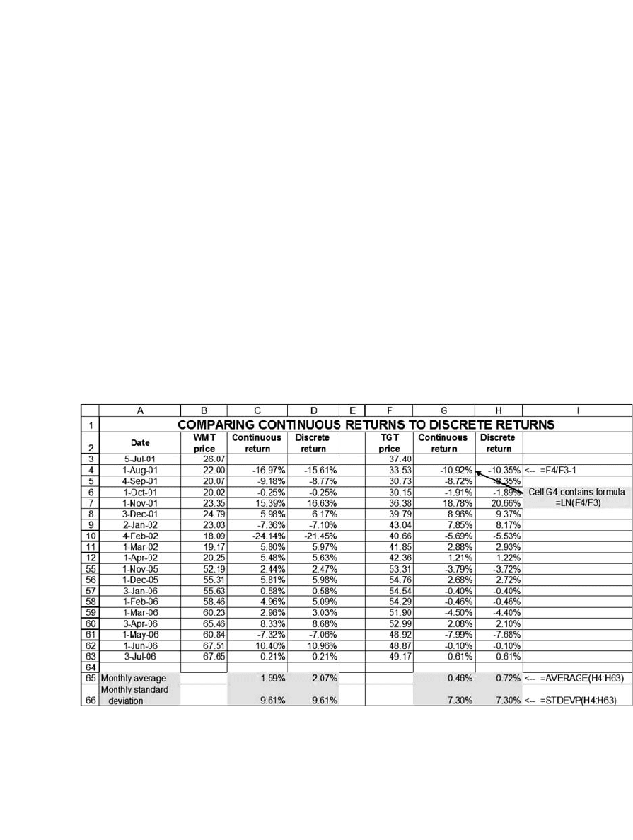
The continuously compounded return will always be smaller than the

discretely compounded return, but the difference is usually not large. The

following table shows the differences for the example in section 8.2:

Calculating Annual Returns and Variances from Periodic Returns

Suppose we calculate a series of continuously compounded monthly

rates of return r

, r

, . . . , r

and we wish to then calculate the mean and

259 Portfolio Models—Introduction

the variance of the annual rate of return. Clearly the mean annual return

is given by

Mean annual return =

⎡

⎣

⎢

⎤

⎦

⎥

∑

To calculate the variance of the annual rate of return, we assume that the

monthly rates of return are independent identically distributed random

variables. It then follows that

Var Var() ()r

monthly

⎡

⎣

⎢

⎤

⎦

⎥

∑

and

that the standard deviation of the annual rate of return is given by

σσ

= 12

monthly

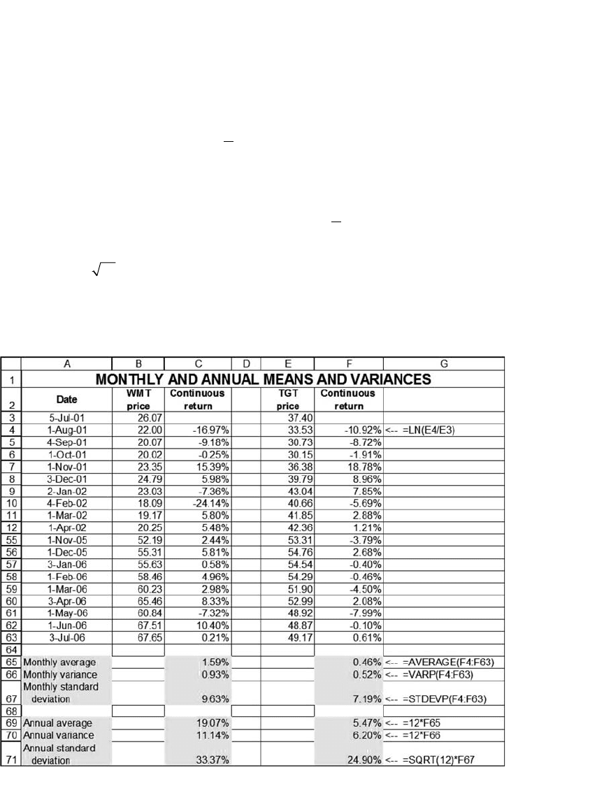
To return to our example: Given our monthly return data, here are the

annual rates of return, their variance, and their standard deviation:

Calculating Efﬁ cient Portfolios When There Are No Short-Sale

Restrictions

9.1 Overview

This chapter covers the theory and calculations necessary for both

versions of the classical capital asset pricing model (CAPM)—both

that which is based on a risk-free asset (also known as the Sharpe-

Lintner-Mossin model) and Black’s (1972) zero-beta CAPM (which

does not require the assumption of a risk-free asset). You will ﬁ nd

that using a spreadsheet enables you to do the necessary calculations

easily.

The structure of the chapter is as follows: We begin with some prelimi-

nary deﬁ nitions and notation. We then state the major results (proofs are

given in the appendix to the chapter). In succeeding sections we imple-

ment these results, showing you

•

How to calculate efﬁ cient portfolios.

•

How to calculate the efﬁ cient frontier.

This chapter includes more theoretical material than most chapters in

this book: Section 9.3 contains the propositions on portfolios that under-

lie the calculations of both efﬁ cient portfolios and the security market

line (SML) in Chapter 11. If you ﬁ nd the theoretical material in section

9.3 difﬁ cult, skip it at ﬁ rst and try to follow the illustrative calculations

in section 9.4. This chapter assumes that the variance-covariance matrix

is given; we delay a discussion of various methods of computing the

variance-covariance matrix until Chapter 10.

9.2 Some Preliminary Deﬁ nitions and Notation

Throughout this chapter we use the following notation: There are N risky

assets, each of which has expected return E(r

). The matrix E(r) is the

column vector of expected returns of these assets:

()

⎡

⎣

⎢

⎤

⎦

⎥



and S is the N × N variance-covariance matrix:

262 Chapter 9

NN NN

⎡

⎣

⎢

⎤

⎦

⎥

σσ σ

11 21 1

12 22 2

...



A portfolio of risky assets (when our intention is clear, we shall just

use the word portfolio) is a column vector x whose coordinates sum to

⎡

⎣

⎢

⎤

⎦

⎥

∑



Each coordinate x

represents the proportion of the portfolio invested in

risky asset i.

The expected portfolio return E(r

) of a portfolio x is given by the

product of x and R:

Er x R xEr

() ()=∗≡

∑

The variance of portfolio x’s return, s

≡ s

is given by the product

xSx xx

ijij

∑∑

The covariance between the return of two portfolios x and y, Cov(r

), is deﬁ ned by the product

σσ

ijij

xSy xy==

∑∑

. Note that s

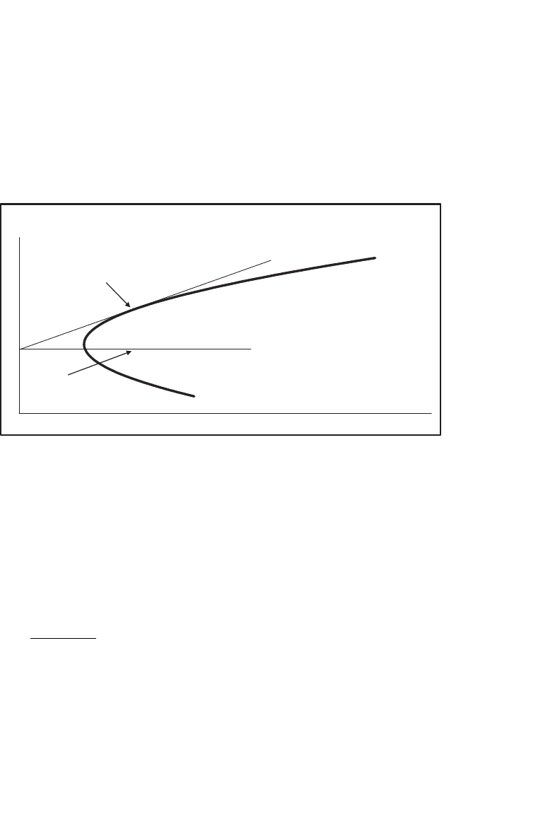
The following graph illustrates four concepts. A feasible portfolio is any

portfolio whose proportions sum to one. The feasible set is the set of

portfolio means and standard deviations generated by the feasible port-

folios; this feasible set is the area inside and to the right of the curved

line. A feasible portfolio is on the envelope of the feasible set if for a given

mean return it has minimum variance. Finally, a portfolio x is an efﬁ cient

portfolio if it maximizes the return given the portfolio variance (or stan-

dard deviation). That is, x is efﬁ cient if there is no other portfolio y such

that E(R

) > E(R

) and s

≤ s

. The set of all efﬁ cient portfolios is called

the efﬁ cient frontier; this frontier is the heavier line in the graph.

263 Calculating Efﬁ cient Portfolios When There Are No Short-Sale Restrictions

9.3 Some Theorems on Efﬁ cient Portfolios and the CAPM

In the appendix to this chapter we prove the following results, which

are basic to the calculations of the CAPM. All these propositions are

used in deriving the efﬁ cient frontier and the security market line;

numerical illustrations are given in the next section and in succeeding

chapters.

proposition 1 Let c be a constant. We use the notation E(r) − c to

denote the following column vector:

Er c

()

−=

−

⎡

⎣

⎢

⎤

⎦

⎥

Let the vector z solve the system of simultaneous linear equations

E(r) − c = Sz. Then this solution produces a portfolio x on the envelope

of the feasible set in the following manner:

Feasible Portfolios

10 20 30 40 50 60 70 80 90

Portfolio standard deviation (%)

Portfolio mean return (%)

Feasible, not

efficient

Envelope, not

efficient

Efficient and

envelope

Infeasible

portfolio

264 Chapter 9

zSEr c

xx x

=−

−1

{() }

{... },,

where

∑

Furthermore, all envelope portfolios are of this form.

Intuition A formal proof of the proposition is given in the appendix to

this chapter, but the intuition is simple and geometric. Suppose we pick

a constant c and we try to ﬁ nd an efﬁ cient portfolio x for which there is

a tangency between c and the feasible set:

Finding Envelope Portfolios

Portfolio standard deviation

Portfolio mean return

x, the tangency

portfolio given c

Proposition 1 gives a procedure for ﬁ nding x; furthermore, the proposi-

tion states that all envelope portfolios (in particular: all efﬁ cient portfo-

lios) are the result of the procedure outlined in the proposition. That is,

if x is any envelope portfolio, then there exists a constant c and a vector

z such that Sz = E(r) − c and

xz z

∑

proposition 2 By a theorem ﬁ rst proved by Black (1972), any two

envelope portfolios are enough to establish the whole envelope. Given

265 Calculating Efﬁ cient Portfolios When There Are No Short-Sale Restrictions

any two envelope portfolios x = {x

, . . . , x

} and y = {y

, . . . , y

}, all enve-

lope portfolios are convex combinations of x and y. This means that given

any constant a, the portfolio

ax a y

+− =

+−

⎡

⎣

⎢

⎤

⎦

⎥

()



is an envelope portfolio.

proposition 3 If y is any envelope portfolio, then for any other portfolio

(envelope or not) x, we have the relationship

Er c Er c

xxy

() [() ]=+ −

where

Cov ,()

Furthermore, c is the expected return of all portfolios z whose covariance

with y is zero:

cEr

= ()

where

Cov ,()yz= 0

Notes If y is on the envelope, the regression of any and all portfolios x

on y gives a linear relationship. In this version of the CAPM (usually

known as Black’s zero-beta CAPM, in honor of Fisher Black, whose 1972

paper proved this result) the Sharpe-Lintner-Mossin security market line

(SML) is replaced with an SML in which the role of the risk-free asset is

played by a portfolio with a zero beta with respect to the particular enve-

lope portfolio y. Note that this result is true for any envelope portfolio y.

The converse of Proposition 3 is also true:

proposition

4 Suppose that there exists a portfolio y such that for any

portfolio x the following relation holds:

266 Chapter 9

Er c Er c

xxy

() [() ]=+ −

where

Cov ,()

Then the portfolio y is an envelope portfolio.

Propositions 3 and 4 show that an SML relation holds if and only if

we regress all portfolio returns on an envelope portfolio. As Roll (1977,

1978) has forcefully pointed out, these propositions show that it is not

enough to run a test of the CAPM by showing that the SML holds.

The

only real test of the CAPM is whether the true market portfolio is mean-

variance efﬁ cient. We shall return to this topic in Chapter 11.

the market portfolio The market portfolio M is a portfolio composed

of all the risky assets in the economy, with each asset taken in proportion

to its value. To make this deﬁ nition more speciﬁ c: Suppose that there are

N risky assets and that the market value of asset i is V

. Then the market

portfolio has the following weights:

Proportion of asset iniM

∑

If the market portfolio M is efﬁ cient (this is a big “if” as we shall see in

Chapters 11 (testing the SML) and 13 (Black-Litterman), Proposition 3

is also true for the market portfolio. That is, the SML holds with E(r

)

substituted for c:

Er Er Er Er

xzxMz

() () [( ) ()]=+ −

where

Cov( , )

Cov( , )zM = 0

1. Roll’s 1977 paper is more cited and more comprehensive, but his 1978 paper is much

easier to read and intuitive. If you’re interested in this literature, start there.

267 Calculating Efﬁ cient Portfolios When There Are No Short-Sale Restrictions

This version of the SML has received the most empirical attention of all

of the CAPM results. In Chapter 11 we show how to calculate b and how

to calculate the SML; we go on to examine Roll’s criticism of these

empirical tests. From the following graph, it is easy to see how to locate

a zero-beta portfolio on the envelope of the feasible set:

Finding Envelope Portfolios

Portfolio standard deviation

Portfolio mean return

x, the tangency

portfolio given c

Zero-beta portfolios

along this line

When there is a risk-free asset, Proposition 3 specializes to the security

market line of the classic capital asset pricing model:

proposition 5 If there exists a risk-free asset with return r

, then there

exists an envelope portfolio x such that

Er r Er r

xfxxf

() [() ]=+ −

where

Cov ,()

As shown in the classic papers by Sharpe (1964), Lintner (1965), and

Mossin (1966), if all investors choose their portfolios only on the basis

of portfolio mean and standard deviation, then the portfolio x of Proposi-

tion 5 is the market portfolio M.

In the remainder of this chapter, we explore the meaning of these

propositions using numerical examples worked out on Excel.