Simon Benninga. Financial Modelling 3-rd edition

Подождите немного. Документ загружается.

248 Chapter 8

proportion in the portfolio; the covariance of each pair of assets appears

once, multiplied by twice the product of the individual assets’ propor-

tions. Another way of writing the variance is to use the notation

Var( ) , Cov( , )rrr

iii ijij

σσ

We may then write

Var( )rxx

jij

∑∑

The most economical representation of the portfolio variance uses

matrix notation. It is also the easiest representation to implement for

large portfolios in Excel. In this representation we call the matrix that

has s

in the ith row and the jth column the variance-covariance

matrix:

NNN

σσσ σ

11 12 13 1

21 22 23 2

31 32 33 3

123

...



NNN

⎡

⎣

⎢

⎤

⎦

⎥

Then the portfolio variance is given by Var(r

) = x

Sx.

If we have two portfolios x = [x

, x

, . . . , x

] and y = [y

, y

, . . . , y

], then

the covariance of the two portfolios is given by Cov(x, y) = xSy

= ySx

8.4.1 Portfolio Calculations Using Matrices—An Example

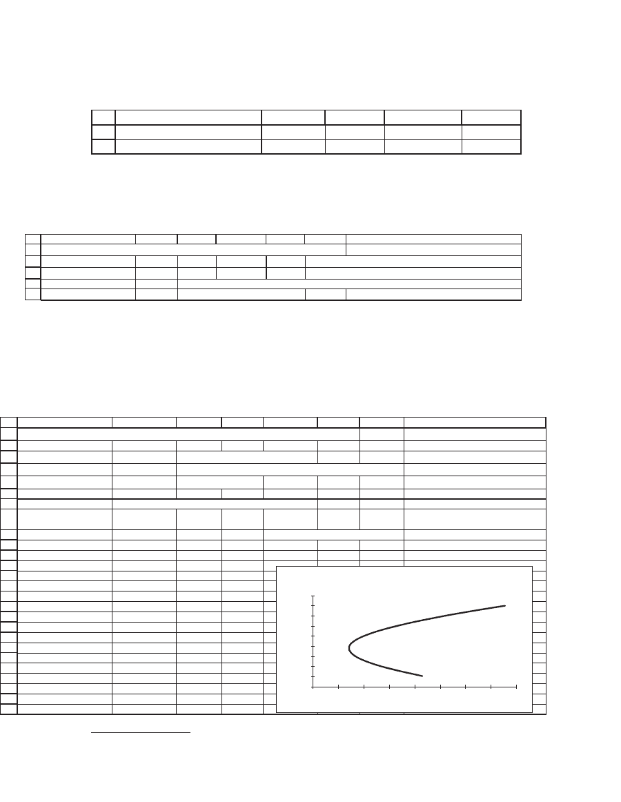
We implement the preceding formulas in a numerical example. Suppose

that there are four risky assets that have the following expected returns

and variance-covariance matrix:

ABCDE

Mean

returns

(r)

0.10 0.01 0.03 0.05 6%

0.01 0.30 0.06 -0.04 8%

0.03 0.06 0.40 0.02 10%

0.05 -0.04 0.02 0.50 15%

Variance-covariance, S

A FOUR-ASSET PORTFOLIO PROBLEM

249 Portfolio Models—Introduction

We consider two portfolios of risky assets:

ABCD

Portfolio x 0.2 0.3 0.4 0.1

Portfolio y 0.2 0.1 0.1 0.6

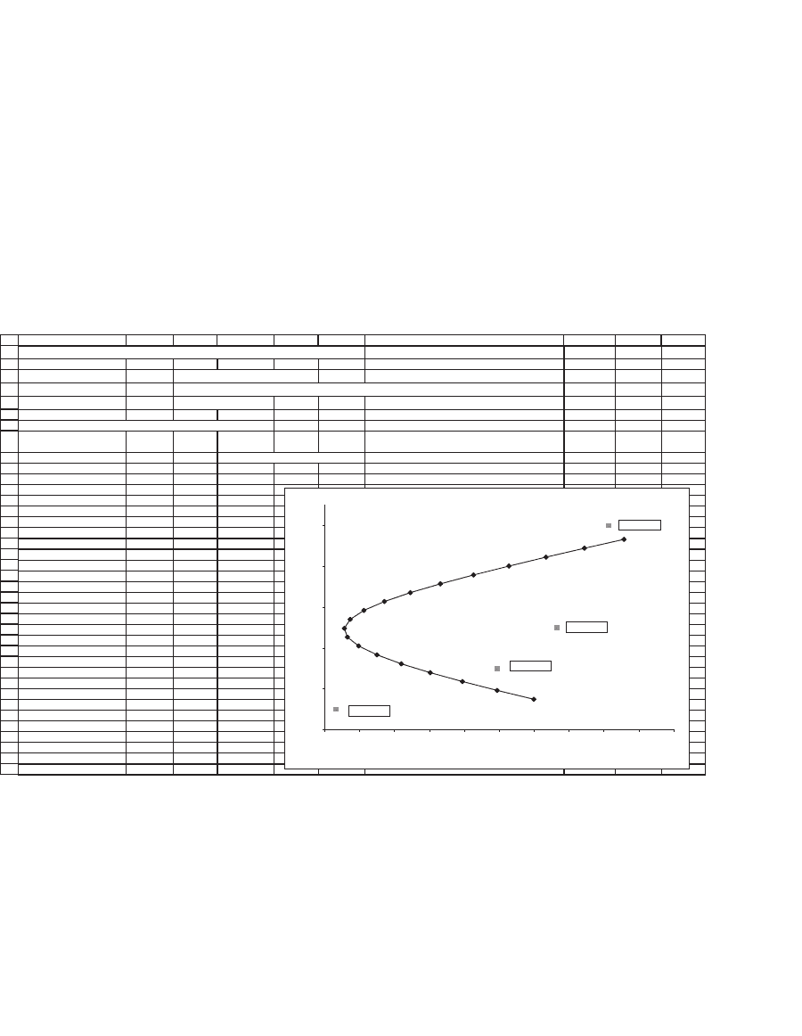
We calculate the means, variances, and covariance of the two portfolios.

We use the Excel array function Mmult for all the calculations and the

array function Transpose to make a row vector into a column vector.

ABCDEF G

Portfolio x and y statistics: Mean, variance, covariance, correlation

Mean, E(r

)

9.10%

Mean, E(r

)

12.00% <-- =MMULT(B9:E9,$F$3:$F$6)

Variance,

0.1216

Variance,

0.2034 <-- =MMULT(B9:E9,MMULT(A3:D6,TRANSPOSE(B9:E9)))

Covariance(x,y) 0.0714 <-- =MMULT(B8:E8,MMULT(A3:D6,TRANSPOSE(B9:E9)))

Correlation,

0.4540 <-- =B14/SQRT(B13*E13)

We can now calculate the standard deviation and return of combina-

tions of portfolios x and y. Note that once we have calculated the means,

variances, and the covariance of the returns of the two portfolios, the

calculation of the mean and the variance of any portfolio is the same as

for the two-asset case.

HGFEDCBA

Calculating returns of combinations of Portfolio X and Portfolio Y

Proportion of Portfolio X 0.3

Mean return, E(r

)

11.13% <-- =B26*C12+(1-B26)*F12

Variance of return, σ

14.06% <-- =B26^2*C13+(1-B26)^2*F13+2*B26*(1-B26)*C15

Stand. dev. of return, σ

37.50% <-- =SQRT(B28)

Table of returns (uses this example and Data|Table)

Proportion

of X

Stand. dev. Mean

37.50% 11.13% <-- Table header: =B29, =B27

0 45.10% 12.00%

0.1 42.29% 11.71%

0.2 39.74% 11.42%

0.3 37.50% 11.13%

0.4 35.63% 10.84%

0.5 34.20% 10.55%

0.6 33.26% 10.26%

0.7 32.84% 9.97%

0.8 32.99% 9.68%

0.9 33.67% 9.39%

1 34.87% 9.10%

1.1 36.53% 8.81%

1.2 38.60% 8.52%

Returns of Combinations of Portfolios X

and Y

10%

11%

12%

13%

30% 32% 34% 36% 38% 40% 42% 44% 46%

Standard deviation

Mean return

3. Remember that MMult and Transpose are array functions and must be entered by

pushing [Ctrl]+[Shift]+[Enter] simultaneously.

250 Chapter 8

8.5 Efﬁ cient Portfolios

An efﬁ cient portfolio is the portfolio of risky assets that gives the lowest

variance of return of all portfolios having the same expected return.

Alternatively, we may say that an efﬁ cient portfolio has the highest

expected return of all portfolios having the same variance. Mathemati-

cally, we may deﬁ ne an efﬁ cient portfolio as follows: For a given return

m, an efﬁ cient portfolio p = [x

, x

, . . . , x

] is one that solves

min ( )xx r

ijij p

∑∑

Var

subject to

xr E r

∑

()

The efﬁ cient frontier is the set of all efﬁ cient portfolios. As shown by

Black (1972), the efﬁ cient frontier is the set of all convex combinations

of any two efﬁ cient portfolios. This statement means that if x = [x

, x

, . . . ,

] and y = [y

, . . . , y

] are efﬁ cient portfolios and if a is a constant,

then the portfolio Z deﬁ ned by

zax ay

ax a y

=+− =

+−

⎡

⎣

⎢

⎤

⎦

⎥

()



is also efﬁ cient. Thus we can ﬁ nd the whole efﬁ cient frontier if we can

ﬁ nd any two efﬁ cient portfolios.

By this theorem, once we have found two efﬁ cient portfolios x and y,

we know that any other efﬁ cient portfolio is a convex combination of x

and y. If we denote the mean and variance of x and y by {E(r

), s

} and

{E(r

), s

}, and if z = ax + (1 − a)y, then

Er aEr aEr

aaaaxy

zx y

() ()( )()

() ()

=+−

=+− +−

121

222 22

σσ σ

Cov( , )

==+− +−aaaaxSy

T22 2 2

121

σσ

() ()

251 Portfolio Models—Introduction

Further details of the calculation of efﬁ cient portfolios are discussed in

Chapter 9.

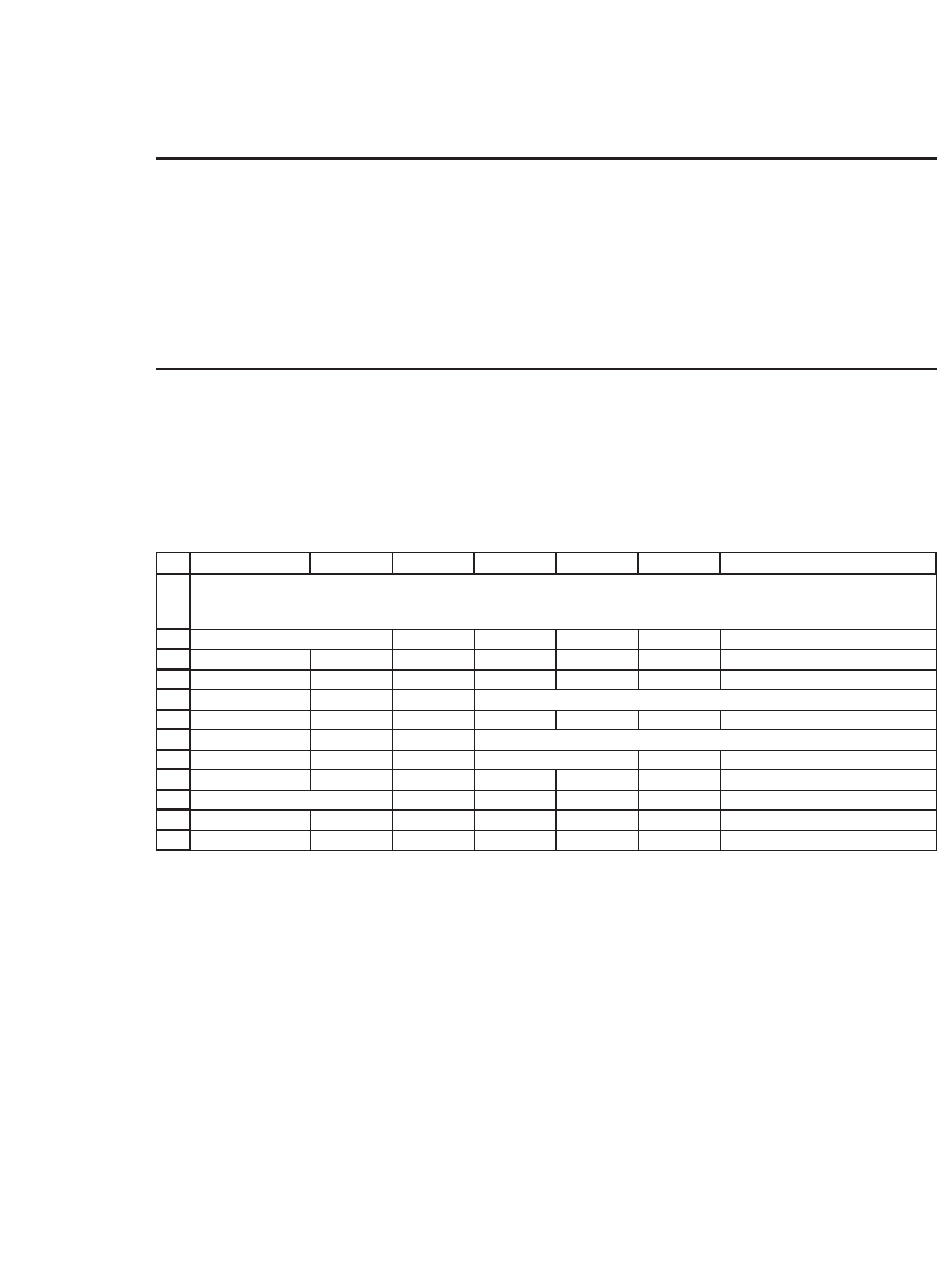
8.5.1 Showing That Portfolios x and y Are Not Efﬁ cient

To show that efﬁ ciency is a nontrivial concept, we show that the two

portfolios whose combinations are graphed in the previous section are

not efﬁ cient. This fact is easy to see if we extend the data table to include

numbers for the individual stocks:

ABCDEF G HI

Calculating returns of combinations of Portfolio x and Portfolio y

Proportion of Portfolio x 0.3

Mean return, E(r

)

11.13% <-- =B18*B12+(1-B18)*E12

Variance of return,

14.06% <-- =B18^2*B13+(1-B18)^2*E13+2*B18*(1-B18)*B14

Stand. dev. of return, σ

37.50% <-- =SQRT(B20)

Table of returns (uses this example and Data|Table)

Proportion

of X

Stand. dev. Mean

37.50% 11.13% <-- Table header: =B21,=B19

-0.80 72.88% 14.32%

-0.65 67.23% 13.89%

-0.50 61.72% 13.45%

-0.35 56.40% 13.02%

-0.20 51.33% 12.58%

-0.05 46.59% 12.15%

0.10 42.29% 11.71%

0.25 38.57% 11.28%

0.40 35.63% 10.84%

0.55 33.66% 10.41%

0.70 32.84% 9.97%

0.85 33.26% 9.54%

1.00 34.87% 9.10%

1.15 37.52% 8.67%

1.30 41.00% 8.23%

1.45 45.13% 7.80%

1.60 49.74% 7.36%

1.75 54.72% 6.93%

1.90 59.96% 6.49%

Stock A 31.62% 6.00%

Stock B 54.77% 8.00%

Stock C 63.25% 10.00%

Stock D 70.71% 15.00%

Portfolios x and y and the Four Stocks

11%

13%

15%

30% 35% 40% 45% 50% 55% 60% 65% 70% 75% 80%

Standard deviation

Mean return

Stock A

Stock D

Stock C

Stock B

Were the two portfolios efﬁ cient, then all of the individual stocks

would fall on or inside the graph of the combinations. In our case, two

of the stock returns (stock A and stock D) fall outside the frontier

created by combinations of portfolios x and y; thus x and y cannot be

efﬁ cient portfolios. In Chapter 9 you will learn to compute efﬁ cient

portfolios, and as you will see there, this task requires considerably more

computation.

252 Chapter 8

8.6 Conclusion

In this chapter we have reviewed the basic concepts and mathematics of

portfolios. In succeeding chapters we shall describe how to compute the

variance-covariance matrix from asset returns and how to calculate efﬁ -

cient portfolios.

Exercises

1. The attached spreadsheet fm3_chapter08.xls includes price data for the Dow-Jones

30 Industrials from July 1997 through July 2007. Isolating the data for Alcoa (AA)

and Johnson & Johnson (JNJ), conﬁ rm the following statistics about the returns of

these two stocks:

ABCDEF G

Monthly statistics AA JNJ

Average 0.68% 0.72% <

=AVERAGE(F16:F135)

Sigma 10.12% 5.84% <

=STDEVP(F16:F135)

Covariance 0.0002 <

=COVAR(C16:C135,F16:F135)

Correlation 0.0398 <

=CORREL(C16:C135,F16:F135)

0.0398 <

=C5/(C4*F4)

Annual statistics AA JNJ

Average 8.11% 8.61% <

=12*F3

Sigma 35.07% 20.24% <

=SQRT(12)*F4

ALCOA (AA) AND JOHNSON & JOHNSON (JNJ)

Return statistics, 1997-2007

2. Using the data from the previous exercise, compute the statistics for each of the

preceding two subperiods, July 1997–July 2002 and July 2002–July 2007.

3. Repeat exercise 2 for Merck (MRK) and Johnson & Johnson (JNJ). Merck had a

big crisis in 2003–2004 related to Vioxx (http://en.wikipedia.org/wiki/Vioxx). Is this

evident in the statistics?

4. Suppose that in July 1997 you bought and held through July 2007 a portfolio com-

posed of 50% Alcoa (AA) and 50% Johnson & Johnson (JNJ) stock.

a. Compute the average monthly return and standard deviation of returns for this

portfolio.

b. Vary the proportion of Alcoa from −1 to 1 and plot the portfolio average returns

as a function of the standard deviation.

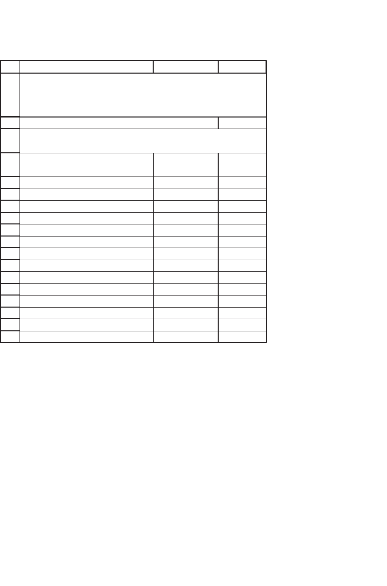
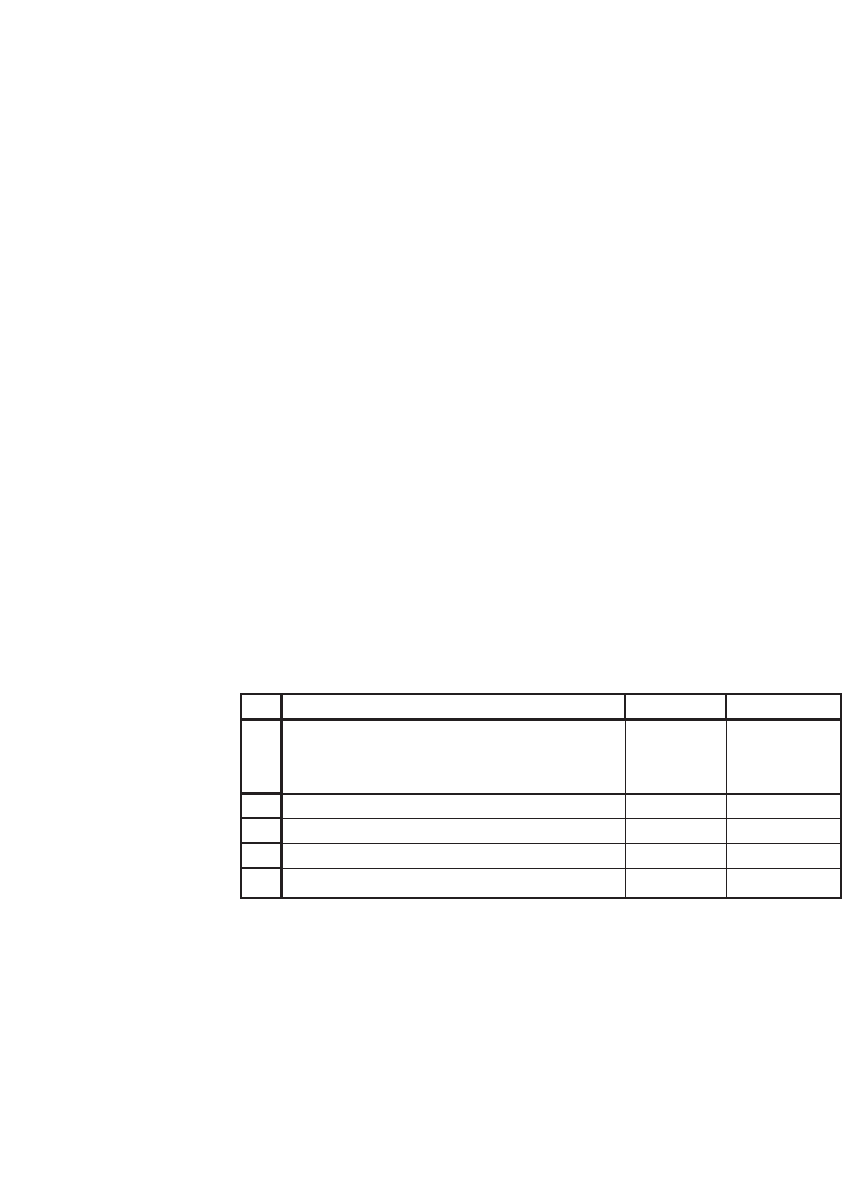
5. Following are annual return statistics for two mutual funds from the Vanguard

family:

253 Portfolio Models—Introduction

Use Excel to graph the combinations of standard deviation of return (x-axis) and

expected return (y-axis) from varying the percentage of Index 500 Fund in the

portfolio from 0% to 100%.

6. Using the database of the DJ Industrials (for 1997–2007), compute for General

Electric (GE), Home Depot (HD), and Procter & Gamble (PG)

a. Average monthly returns

b. Covariances of the monthly returns

c. Monthly expected return and monthly standard deviation of a portfolio that is

equally invested in the three stocks

7. Suppose that X and Y are two random variables and that Y = X

. Let X have values

−5, −4, −2, 2, 4, 5 with equal probabilities. Show that the correlation coefﬁ cient

between X and Y is zero. Does this fact mean that X and Y are independent random

variables?

8. Consider two assets, A and B, that have the following means and variances:

Er Er

() . () .

() . .

003 005

0 0025 0 0045

Var , Var( )

Source: http://www.vanguard.com

Year ended

31 December

Index 500

Fund

Windsor

Fund

1997 33.40% 22.00%

1996 23.00% 26.40%

1995 37.60% 30.10%

1994 1.30% -0.10%

1993 10.10% 19.40%

1992 7.60% 16.50%

1991 30.50% 28.60%

1990 -3.10% -15.50%

1989 31.70% 15.00%

1988 16.60% 28.70%

1987 5.30% 1.20%

1986 18.70% 20.30%

1985 31.80% 28.00%

1984 6.30% 19.50%

Vanguard's Windsor Fund and Index

500 Fund Returns

The Index 500 fund mimics the SP500 index; the

Windsor Fund is an "aggressive" growth fund

254 Chapter 8

Now consider three cases:

ρρρ

AB AB AB

=+ =− =110,,.

Graph the combinations of portfolio means and variances for each case. (Graphs

like these appear in virtually all elementary ﬁ nance books. The standard deviation

usually appears on the x-axis and the portfolio mean return on the y-axis. In this

case, if you want to put all three graphs on the same set of axes, you will have to

reverse this arrangement or use a trick.)

9. Consider a three-asset world with the following parameters:

Mean returns

, Variance-covariance matrix=

⎛

⎝

⎜

⎞

⎠

⎟

003 002 005

00204006

005 006 06

.. .

...

.. .

−

⎛

⎝

⎜

⎞

⎠

⎟

Suppose you have two portfolios with the following portfolio weights:

Portfolio

1030205

2050401

()

...

a. Calculate the mean and variance of each portfolio’s returns and the covariance

and correlation coefﬁ cient of the portfolios’ returns.

b. Create a graph of the means and variance of convex combinations of the

portfolios.

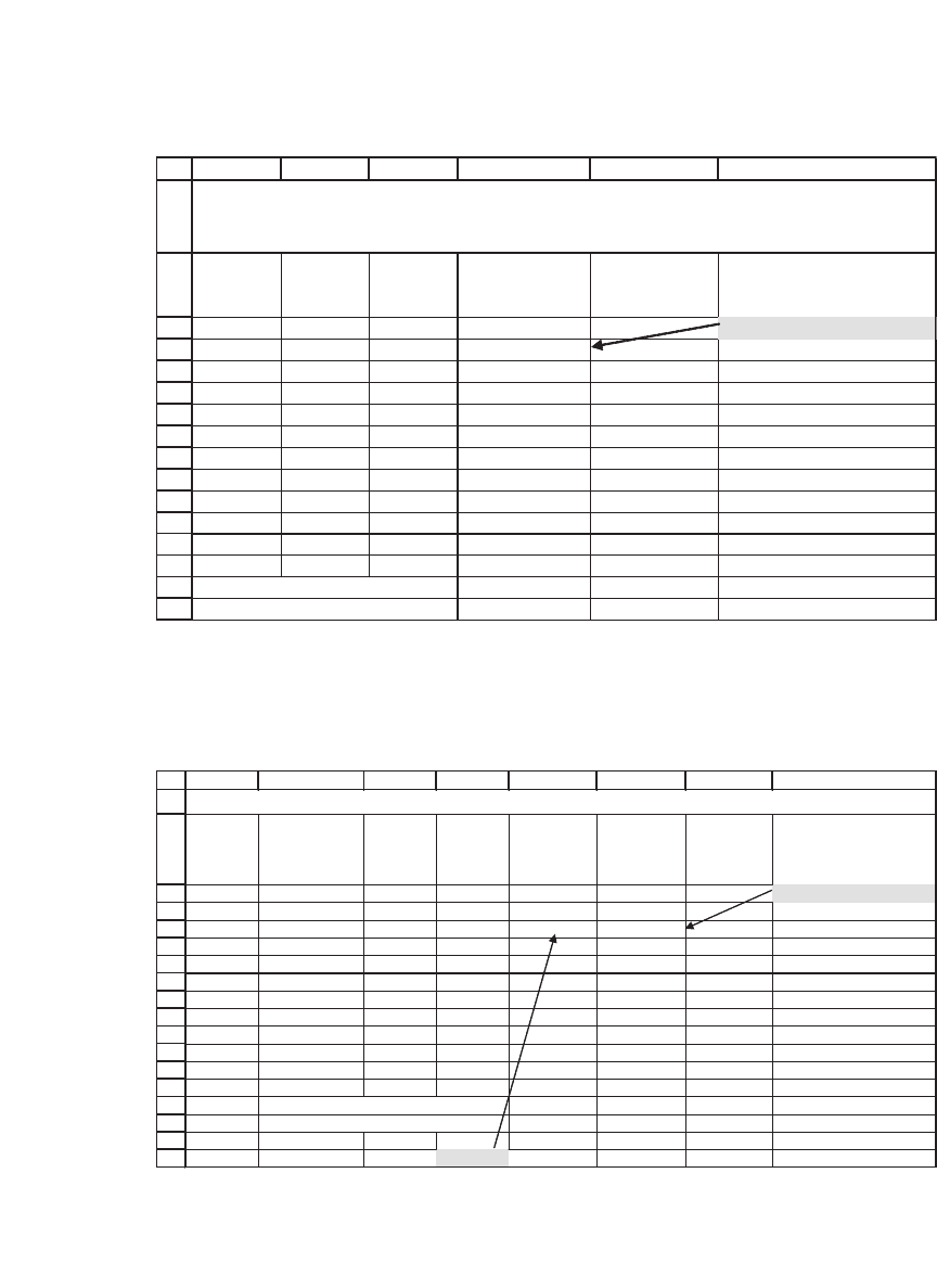
10. In the following spreadsheet, implement the correct formula for cell B12 so that the

portfolio gives the target return indicated in cell B10:

Mean

return

Standard

deviation

of return

Stock 1 12% 35%

Stock 2 18% 50%

Covariance(r

)

0.08350

11. Using the data in the previous exercise, ﬁ nd two portfolios whose standard deviation

of returns is 45%. (There’s an analytical solution to this problem, but it can also be

solved by Solver.)

255 Portfolio Models—Introduction

Appendix 1: Adjusting for Dividends

When downloading data from Yahoo or other sources, the “adjusted

price” includes an adjustment for dividends. In this appendix we discuss

two ways of making this adjustment.

The ﬁ rst, and simplest, method of

adjusting for dividends is to add them to the annual change in price. In

the following example, if you purchased GM stock at the 1986 year-end

price of $33 per share and held it for one year, you would, at the end of

the year, have made 0.57 percent.

Discretely compounded return, per1987

30 69 2 50

33 00

1 0 568=

−=

.ccent

The continuously compounded return is calculated by

Continuously compounded return, 1987

30 69 2 50

33 00

⎡

⎣

⎢

⎤

⎦

⎥

00 567.percent

(The choice between discrete and continuous compounding is discussed

in appendix 2.)

4. It might be argued that since the free sources available on the Web make these adjust-

ments automatically, the details in this appendix are superﬂ uous. Nevertheless we think

they offer some interesting insights. (If you disagree, turn the page!)

256 Chapter 8

ABC D E F

Year

price at

end year

Dividend

per share

Discretely

compounded

return

Continuously

compounded

return

1986 33.00 =(B4+C4)/B3-1

1987 30.69 2.50 0.57% 0.57%

1988 41.75 2.50 44.20% 36.60%

1989 42.25 3.00 8.38% 8.05% <-- =LN((C4+B4)/B3)

1990 34.38 3.00 -11.54% -12.26%

1991 28.88 1.60 -11.35% -12.04%

1992 32.25 1.40 16.54% 15.30%

1993 54.88 0.80 72.64% 54.60%

1994 42.13 0.80 -21.78% -24.56%

1995 52.88 1.10 28.13% 24.79%

1996 55.75 1.60 8.46% 8.12%

Arithmetic annual return

13.43% 9.92% <-- =AVERAGE(E4:E13)

Standard deviation of returns

27.15% 22.84% <-- =STDEVP(E4:E13)

GENERAL MOTORS (GM) STOCK

ADJUSTING FOR DIVIDENDS

GH IJKLM N

Year

Effective

shares held at

beginning of

year

price at

end year

Dividend

per share

Total

dividends

received

Number

of shares at

end of year

Value of

shares at

end of year

1986 33.00 33.000 =H5+K5/I5

1987 1.00 30.69 2.500 2.500 1.081 33.188

1988 1.08 41.75 2.500 2.704 1.146 47.855 <-- =L5*I5

1989 1.15 42.25 3.000 3.439 1.228 51.867

1990 1.23 34.38 3.000 3.683 1.335 45.882

1991 1.33 28.88 1.600 2.136 1.409 40.677

1992 1.41 32.25 1.400 1.972 1.470 47.403

1993 1.47 54.88 0.800 1.176 1.491 81.835

1994 1.49 42.13 0.800 1.193 1.520 64.014

1995 1.52 52.88 1.100 1.672 1.551 82.021

1996 1.55 55.75 1.600 2.482 1.596 88.963

Annualized continous return 9.92% <-- =LN(M13/M3)/10

Compound geometric return

10.43% <-- =(M13/M3)^(1/10)-1

=H5*J5

GM: REINVESTING THE DIVIDENDS IN SHARES

Dividend Reinvestment

Another way of calculating returns is to assume that the dividends are

reinvested in the stock:

Consider ﬁ rst 1987: Since we purchased the share at the end of 1986,

we own one share at the end of 1987. If the 1987 dividend is turned into

257 Portfolio Models—Introduction

shares at the end of 1987 price, we can use it to buy 0.081 additional

New shares purchased at end of 1987

250

30 69

0 081==

Thus we start 1988 with 1.081 shares. Since the 1988 dividend per share

is $2.50, the total dividend received on the shares is 1.081 ∗ $2.50 = $2.704.

Reinvesting these dividends in shares gives

New shares purchased at end of 1988

2 704

41 75

0 065==

Thus, at the end of 1988, the holder of GM shares will have accumulated

1 + 0.081 + 0.065 = 1.146 shares.

As the spreadsheet fragment shows, this reinvestment of dividends will

produce a holding of 1.596 shares at the end of 1996, worth $88.963.

We can calculate the return on this investment in one of two ways:

Continuously compounded return

End- value

Beginning inves

= ln

1996

ttment

percent

⎡

⎣

⎢

⎤

⎦

⎥

⎡

⎣

⎢

⎤

⎦

⎥

88 963

33 00

10 9 92ln

Note that this continuously compounded return (the method preferred

in this book) is the same as that calculated in the ﬁ rst spreadsheet frag-

ment in this appendix from the annual returns (cell E15).

An alternative is to calculate the geometric return:

Compound geometric return

End- value

Initial investment

⎡

⎣

⎢

⎤

1996

⎦⎦

⎥

−

⎡

⎣

⎢

⎤

⎦

⎥

−=

110

88 963

33 00

11043

.percent

Appendix 2: Continuously Compounded versus Geometric Returns

Using the continuously compounded return assumes that P

= P

t−1

, where

is the rate of return during the period (t − 1, t). Suppose that r

, r

, . . . , r

are the returns for 12 periods (a period could be a month or it could be a

year), then the price of the stock at the end of the 12 periods will be