Simon Benninga. Financial Modelling 3-rd edition

Подождите немного. Документ загружается.

268 Chapter 9

9.4 Calculating the Efﬁ cient Frontier: An Example

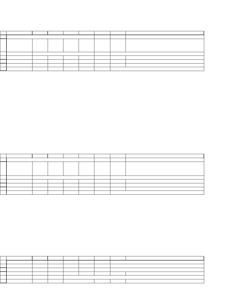
In this section we calculate the efﬁ cient frontier using Excel. We consider

a world with four risky assets having the following expected returns and

variance-covariance matrix:

ABCDEFG H

Expected

returns

E(r)

Expected

minus

constant

E(r) - c

0.40 0.03 0.02 0.00 0.06 0.02 <-- =F3-$B$8

0.03 0.20 0.00 -0.06 0.05 0.01 <-- =F4-$B$8

0.02 0.00 0.30 0.03 0.07 0.03 <-- =F5-$B$8

0.00 -0.06 0.03 0.10 0.08 0.04 <-- =F6-$B$8

Constant 0.04

Variance-covariance matrix

CALCULATING THE EFFICIENT FRONTIER

Each cell of the column vector labeled Expected minus constant contains

the mean return of the given asset minus the value of the constant c (in

this case c = 0.04). We will use this column in ﬁ nding the second envelope

portfolio.

We separate our calculations into two parts: In section 9.4.1 we calcu-

late two portfolios on the envelope of the feasible set. In section 9.4.2

we calculate the efﬁ cient frontier.

9.4.1 Calculating Two Envelope Portfolios

By Proposition 2, we have to ﬁ nd two efﬁ cient portfolios in order to

identify the whole efﬁ cient frontier. By Proposition 1 each envelope

portfolio solves the system R − c = Sz for z. To identify two efﬁ cient

portfolios, we use two different values for c. For each value of c, we solve

for z and then set

xz z

ii h

∑

to ﬁ nd an efﬁ cient portfolio.

The c’s we solve for are arbitrary (see section 9.5), but to make life

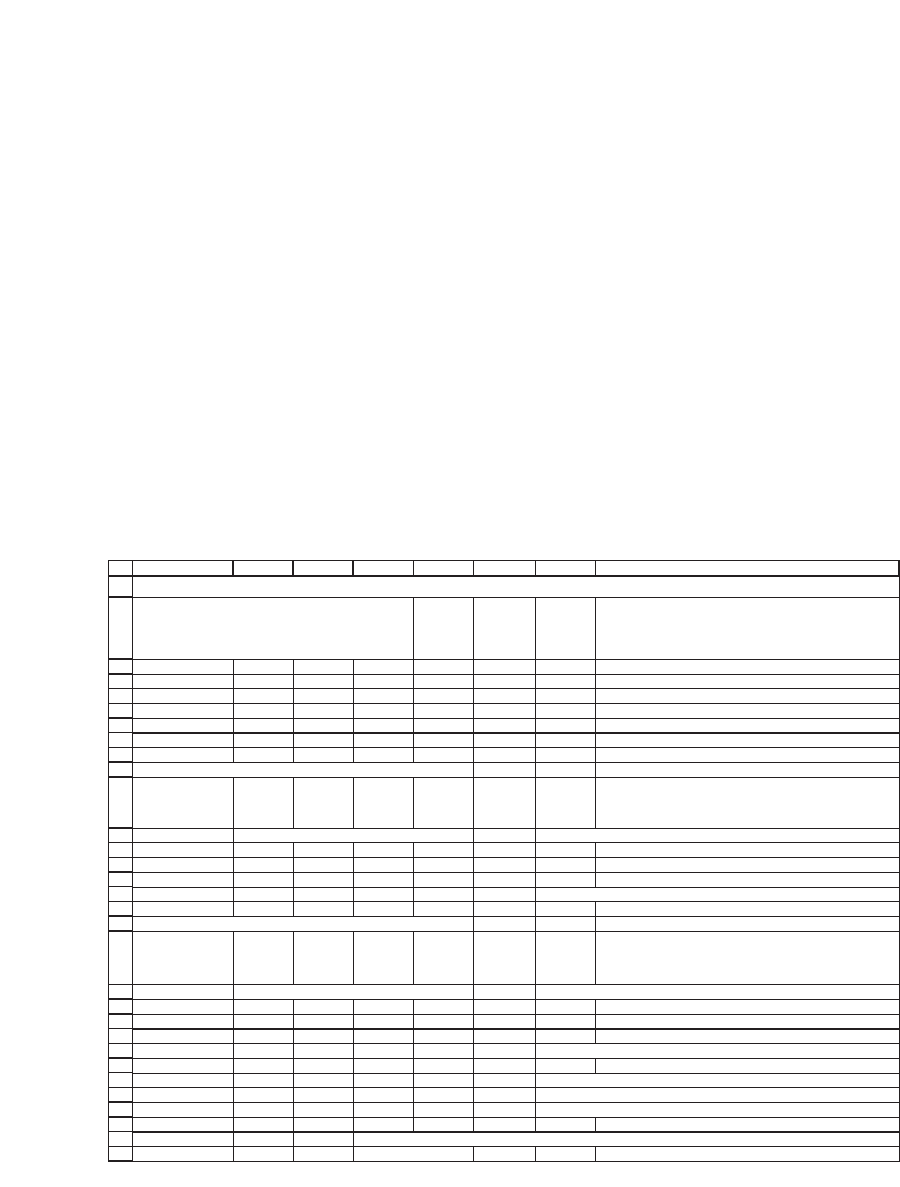
easy, we ﬁ rst solve this system for c = 0. This procedure gives the follow-

ing results:

269 Calculating Efﬁ cient Portfolios When There Are No Short-Sale Restrictions

The formulas in the cells are as follows:

•

For z we use the array function MMult(MInverse(A3 : D6),F3 : F6). The

range A3 : D6 contains the variance-covariance matrix and the cells

F3 : F6 contain the expected returns of the assets.

•

For x: Each cell contains the associated value of z divided by the sum

of all the z’s. Thus, for example, cell F12 contains the formula =A12/SUM

($A$12:$A$15).

To ﬁ nd the second envelope portfolio we now solve this system for

c = 0.04 (cell B8).

ABCDEFG H

Computing an envelope portfolio with constant = 0

Envelope

portfolio

0.1019 <-- {=MMULT(MINVERSE(A3:D6),F3:F6)} 0.0540 <-- =A12/SUM($A$12:$A$15)

0.5657 0.2998

0.1141 0.0605

1.1052 0.5857

Sum 1.0000 <-- =SUM(F12:F15)

ABCDEFG H

Computing an envelope portfolio with constant = 0.04

Envelope

portfolio

0.0330 <-- {=MMULT(MINVERSE(A3:D6),G3:G6)} 0.0423 <-- =A20/SUM($A$20:$A$23)

0.1959 0.2514

0.0468 0.0601

0.5035 0.6462

Sum 1.0000 <-- =SUM(F20:F23)

The portfolio y in cells F20 : F23 is, by the results of Proposition 1, an

envelope portfolio. This vector z associated with y is calculated in a

manner similar to that of the ﬁ rst vector, except that the array function

in the cells is MMult(MInverse(A3 : D6),G3 : G6), where G3 : G6 contains

the vector of expected returns minus the constant 0.04.

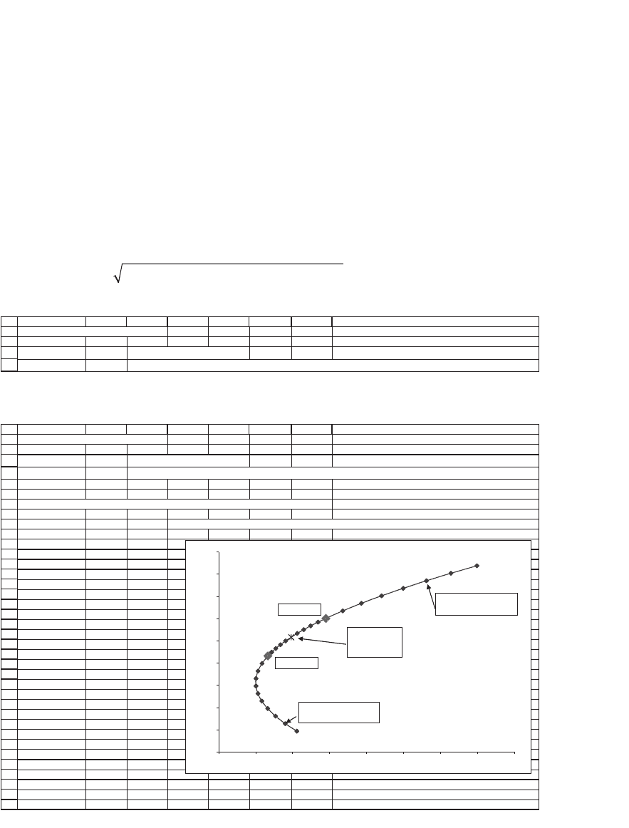
To complete the basic calculations, we compute the means, standard

deviations, and covariance of returns for portfolios x and y:

ABCDEFG H

E(x)

0.0693

E(x)

0.0710 <-- {=MMULT(TRANSPOSE(F20:F23),F3:F6)}

Var(x)

0.0367

Var(y)

0.0398 <-- {=MMULT(MMULT(TRANSPOSE(F20:F23),A3:D6),F20:F23)}

Sigma(x)

0.1917

Sigma(y)

0.1995 <-- =SQRT(F27)

Cov(x,y)

0.0376 <-- {=MMULT(MMULT(TRANSPOSE(F12:F15),A3:D6),F20:F23)}

Corr(x,y)

0.9842 <-- =C30/(B28*F28)

270 Chapter 9

The transpose vectors of x and of y are inserted using the array function

Transpose (see Chapter 35 for a discussion of array functions). This step

now enables us to calculate the mean, variance, and covariance as

follows:

E(x) uses the array formula MMult(transpose_x,means). Note that we

could have also used the function SumProduct(x,means).

Var(x) uses the array formula MMult(MMult(transpose_x,var_cov),x).

Sigma(x) uses the formula Sqrt(var_x).

Cov(x,y) uses the array formula MMult(MMult(transpose_x,var_

cov),y).

Corr(x,y) uses the formula cov(x,y)/(sigma_x*sigma_y).

The following spreadsheet illustrates everything that has been done in

this subsection:

ABCDEFG H

Expected

returns

E(r)

Expected

minus

constant

E(r) - c

0.40 0.03 0.02 0.00 0.06 0.02 <-- =F3-$B$8

0.03 0.20 0.00 -0.06 0.05 0.01 <-- =F4-$B$8

0.02 0.00 0.30 0.03 0.07 0.03 <-- =F5-$B$8

0.00-0.060.030.10 0.080.04<-- =F6-$B$8

Constant 0.04

Computing an envelope portfolio with constant = 0

Envelope

portfolio x

0.1019 <-- {=MMULT(MINVERSE(A3:D6),F3:F6)} 0.0540 <-- =A12/SUM($A$12:$A$15)

0.5657 0.2998

0.1141 0.0605

1.1052 0.5857

Sum 1.0000 <-- =SUM(F12:F15)

Computing an envelope portfolio with constant = 0.04

Envelope

portfolio y

0.0330 <-- {=MMULT(MINVERSE(A3:D6),G3:G6)} 0.0423 <-- =A20/SUM($A$20:$A$23)

0.1959 0.2514

0.0468 0.0601

0.5035 0.6462

Sum 1.0000 <-- =SUM(F20:F23)

E(x)

0.0693

E(x)

0.0710 <-- {=MMULT(TRANSPOSE(F20:F23),F3:F6)}

Var(x)

0.0367

Var(y)

0.0398 <-- {=MMULT(MMULT(TRANSPOSE(F20:F23),A3:D6),F20:F23)}

Sigma(x)

0.1917

Sigma(y)

0.1995 <-- =SQRT(F27)

Cov(x,y)

0.0376 <-- {=MMULT(MMULT(TRANSPOSE(F12:F15),A3:D6),F20:F23)}

Corr(x,y)

0.9842 <-- =C30/(B28*F28)

Variance-covariance matrix

CALCULATING THE EFFICIENT FRONTIER

271 Calculating Efﬁ cient Portfolios When There Are No Short-Sale Restrictions

9.4.2 Calculating the Efﬁ cient Frontier

By Proposition 2 of section 9.3, convex combinations of the two portfo-

lios calculated in the previous subsection allow us to calculate the whole

envelope of the feasible set (which, of course, includes the efﬁ cient fron-

tier). Suppose we let p be a portfolio that has proportion a invested in

portfolio x and proportion (1 − a) invested in y. Then—as discussed in

Chapter 8—the mean and standard deviation of p’s return are

Er aEr aEr

aaaaxy

px y

() ()( )()

() ()()

=+−

=+−+−

121

22 2 2

σσ σ

Cov ,

Here’s a sample calculation for our two portfolios:

ABCDEFG H

A single portfolio calculation

Proportion of x 0.3

E(r

)

7.05% <-- =B35*B26+(1-B35)*F26

19.65% <-- =SQRT(B35^2*B27+(1-B35)^2*F27+2*B35*(1-B35)*C30)

We can turn this calculation into a data table (see Chapter 31) to get the

following table:

ABCDEFG H

A single portfolio calculation

Proportion of x 0.3

E(r

)

7.05% <-- =B35*B26+(1-B35)*F26

19.65% <-- =SQRT(B35^2*B27+(1-B35)^2*F27+2*B35*(1-B35)*C30)

Data table: we vary the proportion of x to produce a graph of the frontier

Proportion of x

Sigma Return

0.1965 0.0705 <-- Data table header refers to cells B36 and B35

-1.400 0.2199 0.0734

-1.200 0.2164 0.0730

-1.000 0.2131 0.0727

-0.800 0.2100 0.0724

-0.600 0.2070 0.0720

-0.400 0.2043 0.0717

-0.200 0.2018 0.0713

0.000 0.1995 0.0710

0.100 0.1984 0.0708

0.200 0.1974 0.0707

0.300 0.1965 0.0705

0.400 0.1956 0.0703

0.500 0.1948 0.0702

0.600 0.1941 0.0700

0.700 0.1934 0.0698

0.800 0.1927 0.0697

0.900 0.1922 0.0695

1.000 0.1917 0.0693

1.200 0.1909 0.0690

1.400 0.1903 0.0686

1.600 0.1901 0.0683

1.800 0.1901 0.0680

2.000 0.1903 0.0676

2.200 0.1908 0.0673

2.400 0.1916 0.0670

2.600 0.1927 0.0666

2.800 0.1940 0.0663

3.000 0.1956 0.0659

0.0650

0.0660

0.0670

0.0680

0.0690

0.0700

0.0710

0.0720

0.0730

0.0740

0.1850 0.1900 0.1950 0.2000 0.2050 0.2100 0.2150 0.2200 0.2250

Portfolio x

Portfolio y

Proportion of x: –1.0

Proportion of y

: 2

Proportion of x: 2.8

Proportion of y

: –1.8

Portfolio w :

50% in x,

50% in y

272 Chapter 9

The two portfolios, x and y, whose convex combinations compose the

envelope are marked, as well as other portfolios, some of which contain

short positions of either x or y. Note that the convex combinations all

lie on the envelope, but may not necessarily be efﬁ cient. For example, w

is an efﬁ cient portfolio that is a convex combination of the two efﬁ cient

portfolios x and y; in this particular case the proportion of x is 50 percent

and that of y is 50 percent. Other envelope portfolios illustrated contain

short positions in one of the two portfolios x and y, and may or may not

be efﬁ cient. Thus, while every efﬁ cient portfolio is a convex combination

of any two efﬁ cient portfolios, it is not true that every convex combina-

tion of any two efﬁ cient portfolios is efﬁ cient.

9.5 Three Notes on the Optimization Procedure

In this section we note three additional facts about the optimization

procedure of Proposition 1 that leads to the computation of envelope

portfolios.

note 1: all roads lead to rome: the precise values of C are irrelevant

for determining the envelope By Proposition 2, the envelope is deter-

mined by any two of its portfolios. Therefore, for the determination of

the envelope it is irrelevant which two portfolios we use. To drive home

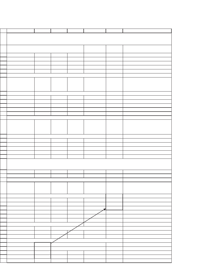
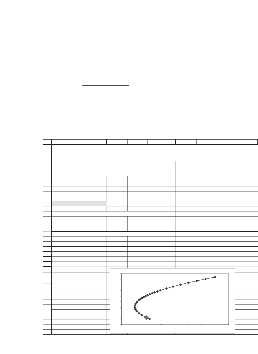
this point, the following spreadsheet computes three envelope

portfolios:

•

The envelope portfolio x is computed with a constant c = −0.03.

•

The envelope portfolio y is computed with a constant c = 0.08.

•

A third envelope portfolio w is computed with a constant c = 0.01

(cells F29 : F32). As shown in rows 36–44, portfolio w is composed of

a convex combination of x and y. This statement is true for any x, y,

and w: the constants c that determine the envelope are completely

arbitrary.

273 Calculating Efﬁ cient Portfolios When There Are No Short-Sale Restrictions

ABCDEF G

Expected

returns

0.40 0.03 0.02 0.00 0.06

0.03 0.20 0.00 -0.06 0.05

0.02 0.00 0.30 0.03 0.07

0.00 -0.06 0.03 0.10 0.08

Computing an envelope portfolio with constant = -0.03

Envelope

portfolio x

0.0502 <-- {=MMULT(MINVERSE(A3:D6),F3:F6-0.03)} 0.0475 <-- {=A10/SUM($A$10:$A$13)}

0.2883 0.2730

0.0636 0.0603

0.6539 0.6192

Sum 1.0000 <-- =SUM(F10:F13)

Computing an envelope portfolio with constant = 0.08

Envelope

portfolio y

-0.0359 <-- {=MMULT(MINVERSE(A3:D6),F3:F6-0.08)} 0.1093 <-- {=A18/SUM($A$18:$A$21)}

-0.1740 0.5293

-0.0205 0.0625

-0.0982 0.2989

Sum 1.0000 <-- =SUM(F18:F21)

Constant 0.01

Computing an envelope portfolio with constant = 0.01

Envelope

portfolio

0.0846 <-- {=MMULT(MINVERSE(A3:D6),F3:F6-B25)} 0.0526 <-- {=A29:A32/SUM(A29:A32)}

0.4732 0.2940

0.0973 0.0604

0.9548 0.5930

Sum 1.0000 <-- =SUM(F29:F32)

Proportions of x and y that determine w

Proportion of x 0.9183 <-- =(F29-F18)/(F10-F18)

Proportion of y 0.0817 <-- =1-B37

Check: Multiply these proportions times portfolios x and y to get w

0.0526 <-- =$B$37*F10+$B$38*F18

0.2940 <-- =$B$37*F11+$B$38*F19

0.0604

0.5930

Variance-covariance matrix

Additional calculation: Fix another constant, and show that the resulting

portfolio is a combination of the two preceding portfolios

CALCULATING THE ENVELOPE

All constants

lead to the same envelope

274 Chapter 9

note 2: certain values of C can also locate envelope portfolios

that are nonefﬁ cient, though they are on the envelope The

optimization procedure of Proposition 1 locates a portfolio x that has

proportions

SEr c

−

{() }

[{()}]Sum

Although always on the envelope, this portfolio is not necessarily efﬁ -

cient, as is shown in the following example, where a constant c = 0.11

leads to an inefﬁ cient portfolio.

ABCDEF G

Expected

returns

E(r)

0.40 0.03 0.02 0.00 0.06

0.03 0.20 0.00 -0.06 0.05

0.02 0.00 0.30 0.03 0.07

0.00 -0.06 0.03 0.10 0.08

Constant 0.11

Computing an envelope portfolio with constant = 0.11

Envelope

portfolio

-0.0876 <-- {=MMULT(MINVERSE(A3:D6),F3:F6-B8)} 0.0755 <-- {=A12:A15/SUM(A12:A15)}

-0.4514 0.3893

-0.0710 0.0613

-0.5495 0.4739

Sum 1.0000 <-- =SUM(F12:F15)

E(r

)

0.0662

0.1944

Variance-covariance matrix

SOME c's CAN LEAD TO INEFFICIENT PORTFOLIOS

The portfolio x determined by the constant c = 0.11 is inefficient

0.065

0.066

0.067

0.068

0.069

0.07

0.071

0.072

0.073

0.074

0.185 0.19 0.195 0.2 0.205 0.21 0.215 0.22 0.225

275 Calculating Efﬁ cient Portfolios When There Are No Short-Sale Restrictions

note 3: if C is the risk-free rate of interest and if the portfolio asso-

ciated with C,

SEr c

−

{() }

{() }Sum[ ]

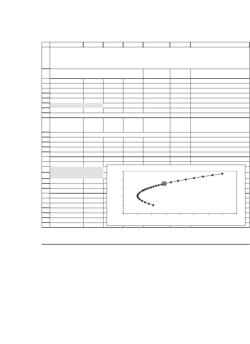
is efﬁ cient, then this portfolio is the optimal portfolio We’ve said

all this before in our discussion of Proposition 1, but it’s worth repeating.

If we set c to be equal to the risk-free rate of interest, and if the resulting

optimizing portfolio

SEr c

−

{() }

{() }Sum[ ]

is efﬁ cient, then this portfolio is the optimal investment portfolio

for an investor whose preferences are deﬁ ned solely in terms of the

mean and standard deviation of portfolio returns. In the following

example we assume that r

= 4 percent. Locating the optimizing

portfolio

SEr c

−

{() }

{() }Sum[ ]

on the envelope shows that it is efﬁ cient. Therefore the optimal invest-

ment portfolio for this case is given by x.

2. And it forms the basis of our discussion of the Black-Litterman model in Chapter 13.

276 Chapter 9

9.6 Finding Efﬁ cient Portfolios in One Step

The examples in section 9.4 ﬁ nd efﬁ cient portfolios by writing out most

of the components of the portfolio separately on the spreadsheet.

However, for some uses we will want to calculate the efﬁ cient portfolio

in one step. Here’s an example:

ABCDEF G

Expected

returns

0.40 0.03 0.02 0.00 0.06

0.03 0.20 0.00 -0.06 0.05

0.02 0.00 0.30 0.03 0.07

0.00 -0.06 0.03 0.10 0.08

Constant 0.04

Computing an envelope portfolio with constant = 0.04

Envelope

portfolio

0.0330 <-- {=MMULT(MINVERSE(A3:D6),F3:F6-B8)} 0.0423 <-- {=A12:A15/SUM(A12:A15)}

0.1959 0.2514

0.0468 0.0601

0.5035 0.6462

Sum 1.0000 <-- =SUM(F12:F15)

E(r

)

0.0710

0.1995

Variance-covariance matrix

IF c = r

AND THE OPTIMIZING PORTFOLIO IS EFFICIENT, THEN THE

ENVELOPE PORTFOLIO IS OPTIMAL

The portfolio

determined by the constant c = 4% is optimal

0.064

0.066

0.068

0.07

0.072

0.074

0.185 0.19 0.195 0.2 0.205 0.21 0.215 0.22 0.225

277 Calculating Efﬁ cient Portfolios When There Are No Short-Sale Restrictions

This approach requires a number of Excel tricks, most of which relate

to the correct use of array functions. The end result is that we can write

the Proposition 1 expression for an envelope portfolio,

SEr c

−

{() }

[{()}]Sum

in one cell:

•

In cells A11 : A14 we have used the array formula F3 : F6-B8 to indicate

the expected returns minus the constant in cell B8.

•

In these same cells we have used SUM(MMULT(MINVERSE(A3 :

D6),F3 : F6-B8)) to give the denominator of the expression

SEr c

−

{() }

{() }Sum[ ]

ABCDEFG H

Expected

returns

E(r)

0.40 0.03 0.02 0.00 0.06

0.03 0.20 0.00 -0.06 0.05

0.02 0.00 0.30 0.03 0.07

0.00 -0.06 0.03 0.10 0.08

Constant 0.05

Envelope

portfolio

0.0314 <-- {=MMULT(MINVERSE(A3:D6),F3:F6-B8)/SUM(MMULT(MINVERSE(A3:D6),F3:F6-B8))}

0.2059

0.0597

0.7031

Portfolio

expected

return, E(r

)

7.26% <-- =SUMPRODUCT(A11:A14,F3:F6)

Portfolio

standard

devation,

21.21% <-- {=SQRT(MMULT(MMULT(TRANSPOSE(A11:A14),A3:D6),A11:A14))}

FINDING EFFICIENT PORTFOLIOS IN ONE STEP

Variance-covariance matrix