Simon Benninga. Financial Modelling 3-rd edition

Подождите немного. Документ загружается.

308 Chapter 10

ABCDEFG H

Return data

Date GE MSFT JNJ K BA IBM

3-Jan-94 56.44% -1.50% 6.01% -9.79% 58.73% 7.74%

3-Jan-95 18.23% 33.21% 41.56% 7.46% -0.24% -12.16%

2-Jan-96 56.93% 44.28% 57.71% 37.76% 65.55% 30.00%

2-Jan-97 42.87% 79.12% 22.94% -5.09% 54.34% -41.78%

2-Jan-98 47.11% 38.04% 17.62% 32.04% 37.11% 47.32%

4-Jan-99 34.55% 85.25% 26.62% -10.74% 15.05% 37.70%

3-Jan-00 28.15% 11.20% 3.41% -48.93% 43.53% -13.32%

2-Jan-01 4.61% -47.19% 10.69% 11.67% 28.29% -78.39%

2-Jan-02 -19.74% 4.27% 23.11% 19.90% -15.09% -25.16%

2-Jan-03 -44.78% -29.47% -5.67% 10.88% -23.23% -137.03%

2-Jan-04 35.90% 18.01% -1.27% 15.49% 39.82% 16.44%

Average 23.66% 21.38% 18.43% 5.51% 27.63% -15.33% <-- =AVERAGE(G4:G14)

Standard deviation 32.17% 40.71% 18.97% 23.86% 29.93% 54.71% <-- =STDEV(G4:G14)

Variance 0.1035 0.1657 0.0360 0.0570 0.0896 0.2993 <-- =VAR(G4:G14)

Constant correlation 0.3000 <-- This is an educated guesstimate

GE MSFT JNJ K BA IBM

0.1035 0.0393 0.0183 0.0230 0.0289 0.0528

MSFT

0.0393 0.1657 0.0232 0.0291 0.0366 0.0668

JNJ

0.0183 0.0232 0.0360 0.0136 0.0170 0.0311

K 0.0230 0.0291 0.0136 0.0570 0.0214 0.0392

0.0289 0.0366 0.0170 0.0214 0.0896 0.0491

IBM

0.0528 0.0668 0.0311 0.0392 0.0491 0.2993

ESTIMATING THE VARIANCE-COVARIANCE MATRIX USING

THE CONSTANT-CORRELATION APPROACH

The constant correlation is set as r = 0.3

Uses the array formula {=IF(A23:A28=B22:G22,B18:G18,MMULT(TRANSPOSE(B17:G17),B17:G17)*B19)} to

compute the constant correlation matrix

10.9 Shrinkage Methods

A third class of methods of estimating the variance-covariance matrix

has recently achieved popularity. So-called shrinkage methods assume

that the variance-covariance matrix is a convex combination of the

sample covariance matrix and some other matrix:

Shrinkage variance-covariance matrix = l

Sample Var-Cov +

(1 − l)

Other matrix

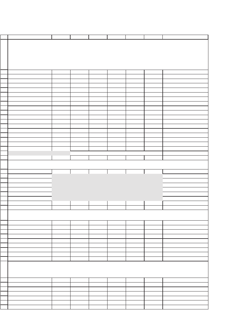
In the following example the “other” matrix is a diagonal matrix of

only variances, with zeros elsewhere. The shrinkage estimator l = 0.3 (cell

B20).

309 Calculating the Variance-Covariance Matrix

ABCDEFG H

Return data

Date GE MSFT JNJ K BA IBM

3-Jan-94 56.44% -1.50% 6.01% -9.79% 58.73% 7.74%

3-Jan-95 18.23% 33.21% 41.56% 7.46% -0.24% -12.16%

2-Jan-96 56.93% 44.28% 57.71% 37.76% 65.55% 30.00%

2-Jan-97 42.87% 79.12% 22.94% -5.09% 54.34% -41.78%

2-Jan-98 47.11% 38.04% 17.62% 32.04% 37.11% 47.32%

4-Jan-99 34.55% 85.25% 26.62% -10.74% 15.05% 37.70%

3-Jan-00 28.15% 11.20% 3.41% -48.93% 43.53% -13.32%

2-Jan-01 4.61% -47.19% 10.69% 11.67% 28.29% -78.39%

2-Jan-02 -19.74% 4.27% 23.11% 19.90% -15.09% -25.16%

2-Jan-03 -44.78% -29.47% -5.67% 10.88% -23.23% -137.03%

2-Jan-04 35.90% 18.01% -1.27% 15.49% 39.82% 16.44%

Average

23.66% 21.38% 18.43% 5.51% 27.63% -15.33% <-- =AVERAGE(G4:G14)

Standard deviation

32.17% 40.71% 18.97% 23.86% 29.93% 54.71% <-- =STDEV(G4:G14)

Variance

0.1035 0.1657 0.0360 0.0570 0.0896 0.2993 <-- =VAR(G4:G14)

Shrinkage factor l

0.3 <-- This is the weight put on the sample var-cov

GE MSFT JNJ K B

A IBM

0.1035 0.0228 0.0066 -0.0013 0.0257 0.0424

MSFT

0.0228 0.1657 0.0124 -0.0016 0.0114 0.0420

JNJ

0.0066 0.0124 0.0360 0.0054 0.0030 0.0137

-0.0013 -0.0016 0.0054 0.0570 -0.0023 0.0037

0.0257 0.0114 0.0030 -0.0023 0.0896 0.0257

IBM

0.0424 0.0420 0.0137 0.0037 0.0257 0.2993

GE MSFT JNJ K BA IBM

0.1035 0.0758 0.0222 -0.0043 0.0857 0.1414

MSFT

0.0758 0.1657 0.0412 -0.0052 0.0379 0.1400

JNJ

0.0222 0.0412 0.0360 0.0181 0.0101 0.0455

-0.0043 -0.0052 0.0181 0.0570 -0.0076 0.0122

0.0857 0.0379 0.0101 -0.0076 0.0896 0.0856

IBM

0.1414 0.1400 0.0455 0.0122 0.0856 0.2993

GE MSFT JNJ K BA IBM

0.1035 0.0000 0.0000 0.0000 0.0000 0.0000

MSFT

0.0000 0.1657 0.0000 0.0000 0.0000 0.0000

JNJ

0.0000 0.0000 0.0360 0.0000 0.0000 0.0000

0.0000 0.0000 0.0000 0.0570 0.0000 0.0000

0.0000 0.0000 0.0000 0.0000 0.0896 0.0000

IBM

0.0000 0.0000 0.0000 0.0000 0.0000 0.2993

ESTIMATING THE VARIANCE-COVARIANCE MATRIX USING

THE SHRINKAGE APPROACH

Gives weight 0.30 (the shrinkage factor) to sample var-cov and

weight 0.70 to a diagonal matrix of only variances

Shrinkage matrix

Uses the array formula {=B20*B34:G39+(1-B20)*B44:G49} to compute the shrinkage covariance matrix

Uses the array formula {=MMULT(TRANSPOSE(B4:G14-B16:G16),B4:G14-B16:G16)/10} to compute the constant

sample covariance matrix. In the shrinkage var-cov, this matrix is given weight lambda.

Uses the array formula {=MMULT(TRANSPOSE(B4:G14-B16:G16),B4:G14-B16:G16)/10*IF(A44:A49=B43:G43,1,0)}

to compute a matrix with only variances on diagonal and zeros elsewhere. In the shrinkage var-cov this matrix is

given weight 1-lambda.

310 Chapter 10

There is little theory about choosing the proper shrinkage estimator.

Our suggestion is to choose a shrinkage operator l so that the GMVP

is wholly positive (see next section for details).

10.10 Alternatives to the Variance-Covariance Matrix: Impact

on the Minimum-Variance Portfolio and the Optimal Portfolio

This chapter has given four alternatives to computing the variance-

covariance matrix:

•

The sample variance-covariance

•

The single-index model

•

The constant-correlation approach

•

Shrinkage methods

How do we compare these alternatives? In this section we compare these

four alternatives on two examples:

•

First, we compute the minimum variance portfolio using each

method.

•

Second, we compute an optimal portfolio using each method.

10.10.1 Minimum Variance Portfolio Using the Sample Variance-Covariance

As its name indicates, the global minimum variance portfolio (GMVP)

is the portfolio that gives the least variance of all portfolios of the assets

under consideration. As shown in section 10.5, the formula for the GMVP

⋅

⋅⋅

−

where S is the variance-covariance portfolio and 1 is a column vector of

1’s.

8. Three papers by Olivier Ledoit and Michael Wolf may offer some guidance: “Improved

Estimation of the Covariance Matrix of Stock Returns with an Application to Portfolio

Selection,” Journal of Empirical Finance, 209, 10, 2003. “A Well-Conditioned Estimator

for Large-Dimensional Covariance Matrices,” Journal of Multivariate Analysis, 88,

2004. “Honey, I Shrunk the Sample Covariance Matrix.” Journal of Portfolio Manage-

ment, 30, 2004.

311 Calculating the Variance-Covariance Matrix

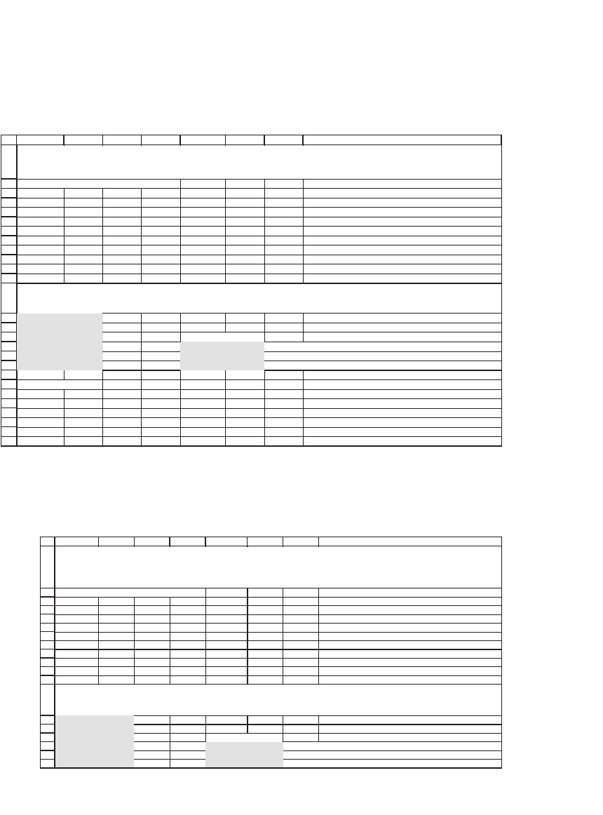
For our sample of six stocks and using the sample variance-covariance

matrix, the GMVP is computed in the following spreadsheet:

ABCDEFG H

Sample variance-covariance matrix

GE MSFT JNJ K BA IBM

GE 0.1035 0.0758 0.0222 -0.0043 0.0857 0.0123

MSFT

0.0758 0.1657 0.0412 -0.0052 0.0379 -0.0022

JNJ 0.0222 0.0412 0.0360 0.0181 0.0101 -0.0039

K -0.0043 -0.0052 0.0181 0.0570 -0.0076 -0.0046

A 0.0857 0.0379 0.0101 -0.0076 0.0896 0.0248

IBM 0.0123 -0.0022 -0.0039 -0.0046 0.0248 0.0184

Average 23.66% 21.38% 18.43% 5.51% 27.63% 17.63%

GE 0.6105

MSFT -0.1034

JNJ 0.2074 GMVP statistics

K 0.0539 Mean return 12.73% <-- {=MMULT(B11:G11,B14:B19)}

-0.7704 Variance 0.0060 <-- {=MMULT(MMULT(TRANSPOSE(B14:B19),B4:G9),B14:B19)}

IBM 1.0019 Sigma 7.73% <-- =SQRT(F18)

Column vector of 1s

GE 1

MSFT 1

JNJ 1

A 1

IBM

Uses formula {=MMULT(MINVERSE(B4:G9),B22:B27)/SUM(MMULT(MINVERSE(B4:G9),B22:B27))}

to compute the global minimum variance portfolio

COMPUTING THE GLOBAL MINIMUM VARIANCE PORTFOLIO USING

THE SAMPLE VAR-COV MATRIX

The GMVP has a mean return of 12.73 percent (cell F17) and standard

deviation of 7.73 percent (cell F19).

There’s a more compact way to do this calculation:

ABCDEFG H

Sample variance-covariance matrix

GE MSFT JNJ K BAIBM

GE 0.1035 0.0758 0.0222 -0.0043 0.0857 0.0123

MSFT 0.0758 0.1657 0.0412 -0.0052 0.0379 -0.0022

JNJ 0.0222 0.0412 0.0360 0.0181 0.0101 -0.0039

K -0.0043 -0.0052 0.0181 0.0570 -0.0076 -0.0046

A 0.0857 0.0379 0.0101 -0.0076 0.0896 0.0248

IBM 0.0123 -0.0022 -0.0039 -0.0046 0.0248 0.0184

Average 23.66% 21.38% 18.43% 5.51% 27.63% 17.63%

GE 0.6105

MSFT

-0.1034

JNJ 0.2074 GMVP statistics

0.0539 Mean return 12.73% <-- {=MMULT(B11:G11,B14:B19)}

A -0.7704 Variance 0.0060 <-- {=MMULT(MMULT(TRANSPOSE(B14:B19),B4:G9),B14:B19)}

IBM

1.0019 Sigma 7.73% <-- =SQRT(F18)

Uses formula {=MMULT(MINVERSE(B4:G9),IF(A14:A19=A14:A19,1,0))/SUM(MMULT(MINVERSE(B4:G9),IF(A14:A19=A14:A19,1,0)))}

to compute the global minimum variance portfolio

COMPUTING THE GLOBAL MINIMUM VARIANCE PORTFOLIO USING THE SAMPLE VAR-COV

MATRIX

More compact method: uses trick to compute vector of 1s

312 Chapter 10

This more compact method uses the array formula If(A14:A19=A14:

A19,1,0) to compute the vector of 1s.

10.10.2 GMVP Using the Alternative Variance-Covariance Matrices

In this subsection we repeat the preceding exercise using three variations

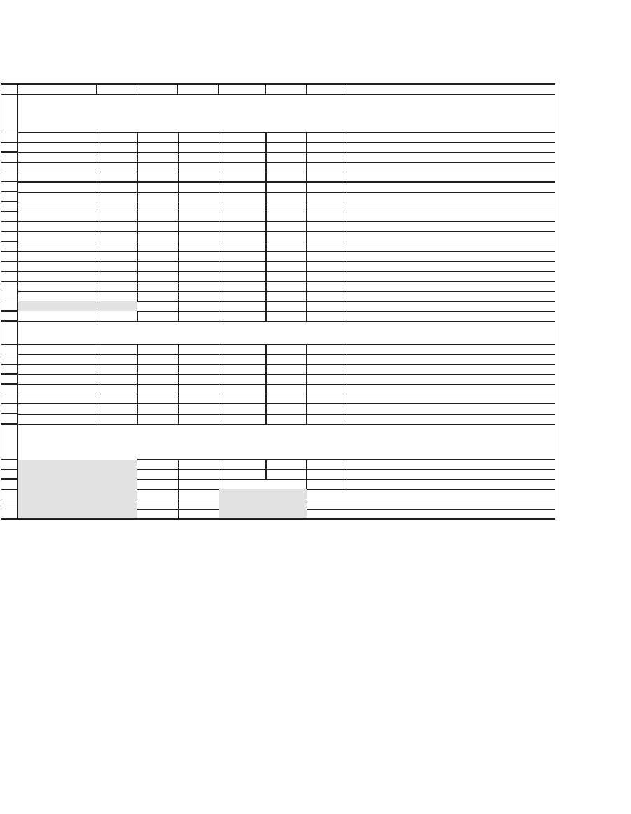
for the variance-covariance matrix. Using the single-index model (SIM)

we get the following GMVP:

ABCDEFG H

Sample variance-covariance matrix

GE MSFT JNJ K B

AIBM

GE 0.1035 0.0120 0.0034 0.0031 0.0014 0.0002

MSFT 0.0120 0.1657 0.0092 0.0083 0.0037 0.0007

JNJ 0.0034 0.0092 0.0360 0.0023 0.0010 0.0002

0.0031 0.0083 0.0023 0.0570 0.0009 0.0002

A 0.0014 0.0037 0.0010 0.0009 0.0896 0.0001

IBM

0.0002 0.0007 0.0002 0.0002 0.0001 0.0184

Average 23.66% 21.38% 18.43% 5.51% 27.63% 17.63%

GE 0.0678

MSFT 0.0251

JNJ 0.2153 GMVP statistics

0.1337 Mean return 17.59% <-- {=MMULT(B11:G11,B14:B19)}

A 0.0907 Variance 0.0087 <-- {=MMULT(MMULT(TRANSPOSE(B14:B19),B4:G9),B14:B19)}

IBM

0.4674 Sigma 9.33% <-- =SQRT(F18)

Uses formula {=MMULT(MINVERSE(B4:G9),IF(A14:A19=A14:A19,1,0))/SUM(MMULT(MINVERSE(B4:G9),IF(A14:A19=A14:A19,1,0)))}

to compute the global minimum variance portfolio

COMPUTING THE GLOBAL MINIMUM VARIANCE PORTFOLIO

USING THE SINGLE-INDEX MODEL

The remarkable change is not the GMVP statistics, but rather the

composition of the GMVP, which is now composed solely of positive

proportions of the stocks.

In the next spreadsheet we use the constant-correlation matrix:

313 Calculating the Variance-Covariance Matrix

ABCDEFG H

Return data

Date GE MSFT JNJ K BAIBM

3-Jan-94 56.44% -1.50% 6.01% -9.79% 58.73% 7.74%

3-Jan-95 18.23% 33.21% 41.56% 7.46% -0.24% -12.16%

2-Jan-96 56.93% 44.28% 57.71% 37.76% 65.55% 30.00%

2-Jan-97 42.87% 79.12% 22.94% -5.09% 54.34% -41.78%

2-Jan-98 47.11% 38.04% 17.62% 32.04% 37.11% 47.32%

4-Jan-99 34.55% 85.25% 26.62% -10.74% 15.05% 37.70%

3-Jan-00 28.15% 11.20% 3.41% -48.93% 43.53% -13.32%

2-Jan-01 4.61% -47.19% 10.69% 11.67% 28.29% -78.39%

2-Jan-02 -19.74% 4.27% 23.11% 19.90% -15.09% -25.16%

2-Jan-03 -44.78% -29.47% -5.67% 10.88% -23.23% -137.03%

2-Jan-04 35.90% 18.01% -1.27% 15.49% 39.82% 16.44%

Average 23.66% 21.38% 18.43% 5.51% 27.63% -15.33% <-- =AVERAGE(G4:G14)

Standard deviation 32.17% 40.71% 18.97% 23.86% 29.93% 54.71% <-- =STDEV(G4:G14)

Variance 0.1035 0.1657 0.0360 0.0570 0.0896 0.2993 <-- =VAR(G4:G14)

Constant correlation 0.3000

GE MSFT JNJ K B

AIBM

GE 0.1035 0.0393 0.0183 0.0230 0.0289 0.0528

MSFT 0.0393 0.1657 0.0232 0.0291 0.0366 0.0668

JNJ 0.0183 0.0232 0.0360 0.0136 0.0170 0.0311

0.0230 0.0291 0.0136 0.0570 0.0214 0.0392

A 0.0289 0.0366 0.0170 0.0214 0.0896 0.0491

IBM 0.0528 0.0668 0.0311 0.0392 0.0491 0.2993

GE 0.0800

MSFT 0.0030

JNJ

0.5645

GMVP statistics

K 0.2782 Mean return 15.97% <-- {=MMULT(B11:G11,B31:B36)}

A 0.1152 Variance 0.4027 <-- {=MMULT(MMULT(TRANSPOSE(B31:B36),B4:G9),B31:B36)}

IBM -0.0409 Sigma 63.46% <-- =SQRT(F35)

Uses formula {=MMULT(MINVERSE(B23:G28),IF(A31:A36=A31:A36,1,0))/SUM(MMULT(MINVERSE(B23:G28),IF(A31:A36=A31:A36,1,0)))} to

compute the global minimum variance portfolio

COMPUTING THE GLOBAL MINIMUM VARIANCE PORTFOLIO

USING CONSTANT CORRELATION MODEL

Uses the array formula {=IF(A23:A28=B22:G22,B18:G18,MMULT(TRANSPOSE(B17:G17),B17:G17)*B19)}

to compute the constant correlation matrix

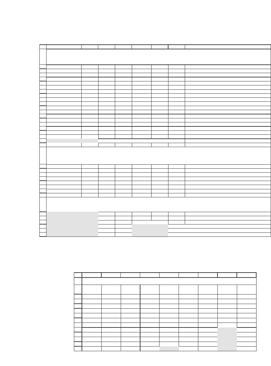
Using the shrinkage variance-covariance matrix, we get the following

results:

314 Chapter 10

ABCDEFG H

Return data

Date GE MSFT JNJ K BAIBM

3-Jan-94 56.44% -1.50% 6.01% -9.79% 58.73% 21.51%

3-Jan-95 18.23% 33.21% 41.56% 7.46% -0.24% 6.04%

2-Jan-96 56.93% 44.28% 57.71% 37.76% 65.55% 27.33%

2-Jan-97 42.87% 79.12% 22.94% -5.09% 54.34% 41.08%

2-Jan-98 47.11% 38.04% 17.62% 32.04% 37.11% 2.63%

4-Jan-99 34.55% 85.25% 26.62% -10.74% 15.05% -2.11%

3-Jan-00 28.15% 11.20% 3.41% -48.93% 43.53% 23.76%

2-Jan-01 4.61% -47.19% 10.69% 11.67% 28.29% 21.76%

2-Jan-02 -19.74% 4.27% 23.11% 19.90% -15.09% 4.55%

2-Jan-03 -44.78% -29.47% -5.67% 10.88% -23.23% 15.54%

2-Jan-04 35.90% 18.01% -1.27% 15.49% 39.82% 31.80%

Average 23.66% 21.38% 18.43% 5.51% 27.63% 17.63% <-- =AVERAGE(G4:G14)

Standard deviation 32.17% 40.71% 18.97% 23.86% 29.93% 13.56% <-- =STDEV(G4:G14)

Variance 0.1035 0.1657 0.0360 0.0570 0.0896 0.0184 <-- =VAR(G4:G14)

Shrinkage factor

0.3 <-- This is the weight put on the sample var-cov

GE MSFT JNJ K B

AIBM

GE 0.1035 0.0228 0.0066 -0.0013 0.0257 0.0037

MSFT 0.0228 0.1657 0.0124 -0.0016 0.0114 -0.0007

JNJ 0.0066 0.0124 0.0360 0.0054 0.0030 -0.0012

K -0.0013 -0.0016 0.0054 0.0570 -0.0023 -0.0014

A 0.0257 0.0114 0.0030 -0.0023 0.0896 0.0074

IBM 0.0037 -0.0007 -0.0012 -0.0014 0.0074 0.0184

GE 0.0407

MSFT 0.0337

JNJ 0.2261 GMVP statistics

K 0.1556 Mean return 14.94% <-- {=MMULT(B11:G11,B32:B37)}

A 0.0412 Variance 0.1967 <-- {=MMULT(MMULT(TRANSPOSE(B32:B37),B4:G9),B32:B37)}

IBM 0.5027 Sigma 44.35% <-- =SQRT(F36)

Uses formula {=MMULT(MINVERSE(B24:G29),IF(A32:A37=A32:A37,1,0))/SUM(MMULT(MINVERSE(B24:G29),IF(A32:A37=A32:A37,1,0)))} to

compute the global minimum variance portfolio

COMPUTING THE GLOBAL MINIMUM VARIANCE PORTFOLIO

USING A SHRINKAGE VARIANCE-COVARIANCE MATRIX

Shrinkage matrix

Uses the array formula {=B20*MMULT(TRANSPOSE(B4:G14-B16:G16),B4:G14-B16:G16)/10+(1-B20)*MMULT(TRANSPOSE(B4:G14-

B16:G16),B4:G14-B16:G16)/10*IF(A24:A29=B23:G23,1,0)}

to compute the shrinkage covariance matrix

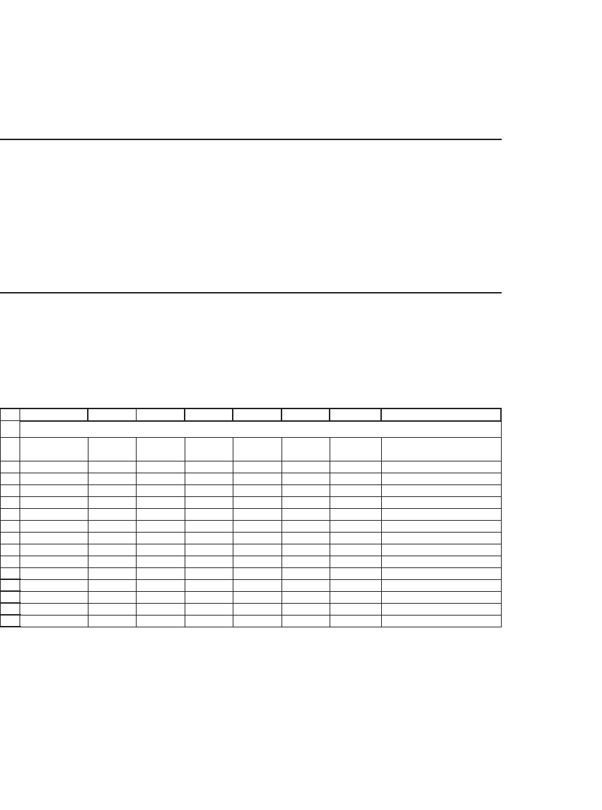
Changing the shrinkage factor alters the GMVP. In the following data

table we vary l from 0 to 1 (when l = 1 the GMVP is the same as that

achieved with the sample variance-covariance matrix):

JKLMNOPQR

GMVP

mean

GMVP

gma

GE MSFT JNJ K BA IBM

0 13.91% 47.53% 0.0763 0.0477 0.2196 0.1387 0.0882 0.4295

0.1 14.33% 46.41% 0.0630 0.0420 0.2216 0.1467 0.0726 0.4541

0.2 14.67% 45.35% 0.0511 0.0374 0.2238 0.1523 0.0571 0.4783

0.3 14.94% 44.35% 0.0407 0.0337 0.2261 0.1556 0.0412 0.5027

0.4 15.13% 43.40% 0.0319 0.0308 0.2287 0.1568 0.0243 0.5274

0.5 15.26% 42.49% 0.0251 0.0286 0.2316 0.1559 0.0055 0.5533

0.6 15.30% 41.60% 0.0214 0.0268 0.2349 0.1528 -0.0168 0.5811

0.7 15.24% 40.71% 0.0232 0.0247 0.2383 0.1470 -0.0457 0.6124

0.8 15.03% 39.68% 0.0379 0.0209 0.2415 0.1378 -0.0894 0.6513

0.9 14.44% 38.06% 0.0952 0.0087 0.2422 0.1217 -0.1807 0.7130

1 10.55% 32.43% 0.6105 -0.1034 0.2074 0.0539 -0.7704 1.0019

Data table: varying the shrinkage factor l

315 Calculating the Variance-Covariance Matrix

We have used Excel’s Conditional Formatting feature to mark all the

portfolios for which there are short sales.

10.11 Summary

In this chapter we considered how to compute the variance-covariance

matrix, which is central to all portfolio optimization. Starting with the

standard sample variance-covariance matrix, we also showed how to

compute several alternatives that have appeared in the literature as

perhaps improving portfolio computations.

Exercises

1. In the following table you will ﬁ nd annual return data for six furniture compa-

nies between the years 1982 and 1992. Use these data to calculate the variance-

covariance matrix of the returns.

ABCDEFG H

La-Z-Boy Kimball Flexsteel

Leggett

& Platt

Herman

Miller

Shaw

Industries

1982

36.67% 0.20% 41.54% 21.92% 26.13% 22.50%

1983

122.82% 61.43% 195.09% 62.27% 73.38% 117.89%

1984

14.44% 63.51% -38.38% -1.27% 45.15% 7.80%

1985

21.39% 28.42% 1.30% 81.17% 24.27% 38.14%

1986

45.36% -7.44% 21.89% 19.83% 10.73% 54.48%

1987

20.19% 48.27% 9.11% -10.21% -11.92% 26.82%

1988

-8.94% -11.28% 12.65% 13.77% 7.06% -6.24%

1989

27.02% 12.85% 12.08% 32.55% -7.55% 123.03%

1990

-11.64% 2.42% -17.13% -6.48% 1.31% 15.48%

1991

20.29% 6.90% 3.62% 50.12% -5.54% 19.92%

1992

34.08% 22.21% 33.46% 84.40% 5.71% 62.76%

Beta

0.80 0.95 0.65 0.85 0.85 1.40

Mean returns

29.24% 20.68% 25.02% 31.64% 15.34% 43.87% <

=AVERAGE(G3:G13)

DATA FOR 6 FURNITURE COMPANIES

2. For the ﬁ rms from the previous example, calculate the variance-covariance matrix

using the single-index model. Assume that the variance of the market portfolio is

18%.

3. In the Excel notebook fm3_problems10.xls on the disk accompanying this book,

you will ﬁ nd monthly price data for the 30 stocks in the Dow-Jones Index of

30 Industrials for July 1997–July 2007. Use this data to compute the variance-

covariance matrix of the DJ30.

316 Chapter 10

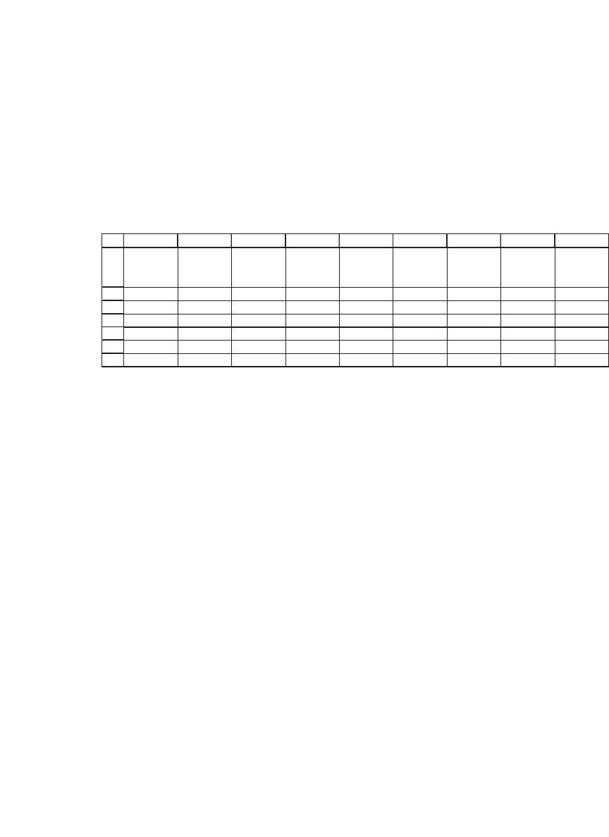
4. The following chart shows the variance-covariance matrix and the mean returns for

six stocks. All the data are for monthly data (raw data are on the disk with the

book).

a. Compute the global minimum variance portfolio (GMVP).

b. Compute the efﬁ cient portfolio, assuming a monthly risk-free rate of 0.45%.

c. Show the frontier as the expected return and standard deviation of convex com-

binations of the GMVP and the efﬁ cient portfolio.

ABCDEFGH I

Kroger

Ford

Target

TGT

Juniper

Networks

JNPR

Ahold

AHO

KeyCorp

KEY

Mean

returns

KR 0.0052 0.0033 0.0015 0.0039 0.0068 0.0010

0.24%

F 0.0033 0.0120 0.0034 0.0072 0.0063 0.0015

-0.89%

TGT 0.0015 0.0034 0.0046 0.0058 0.0039 0.0015

0.48%

JNPR

0.0039 0.0072 0.0058 0.0379 0.0073 0.0023 0.44%

AHO

0.0068 0.0063 0.0039 0.0073 0.0389 0.0023 -1.46%

KEY

0.0010 0.0015 0.0015 0.0023 0.0023 0.0018 1.04%

5. Repeat the preceding exercise when the variance-covariance matrix is an equally

weighted combination of the sample matrix in exercise 4 and a pure diagonal matrix

of only the variances.

Estimating Betas and the Security Market Line

11.1 Overview

The capital asset pricing model (CAPM) is one of the two most inﬂ uential

innovations in ﬁ nancial theory in the latter half of the twentieth century.

By integrating the portfolio decision with utility theory and the statistical

behavior of asset prices, the formulators of the CAPM deﬁ ned the para-

digm that is now generally used for the analysis of stock prices.

What does the CAPM actually say? What are its empirical implica-

tions? Roughly speaking, we can differentiate between two kinds of

implications of the CAPM. First, the capital market line (CML) deﬁ nes

the individual optimal portfolios for an investor interested in the mean

and variance of her optimal portfolio. Second, given agreement between

investors on the statistical properties of asset returns and on the impor-

tance of mean-variance optimization, the security market line (SML)

deﬁ nes the risk-return relation for each individual asset.

It is useful to differentiate between the case where a risk-free asset

exists and the case where there is no risk-free asset.

11.1.1 Case 1: A Risk-Free Asset Exists

Suppose a risk-free asset exists and has return r

. We can differentiate

between the individual optimization of investors and the general equi-

librium implications of the CAPM:

•

Individual optimization: Assuming that investors optimize based on the

expected return and standard deviation of their portfolio returns (in the

jargon of ﬁ nance—they have “mean-variance” preferences), the CAPM

states that each individual investor’s optimal portfolio falls on the line

E(r

) = r

+ s

[E(r

) − r

], where portfolio x is a portfolio that maximizes

Er r

()−

for all feasible portfolios y. Proposition 1 of Chapter 9 shows

1. The other remarkable innovation is option-pricing theory, which is discussed in Chap-

ters 16–24. These two innovations together have accounted for a number of Nobel

prizes in economics: Harry Markowitz (1990), William Sharpe (1990), Myron Scholes

(1997), Robert Merton (1997). But for their untimely demise, others associated with

these theories—Jan Mossin (1936–87) and Fisher Black (1938–95)—would doubtless

also have received the Nobel.

2. The existence (or nonexistence) of a risk-free asset is closely related to the investment

horizon. Assets that are risk-free over a short term may not be riskless over a longer

term.