Seuront L. Fractals and Multifractals in Ecology and Aquatic Science

Подождите немного. Документ загружается.

114 Fractals and Multifractals in Ecology and Aquatic Science

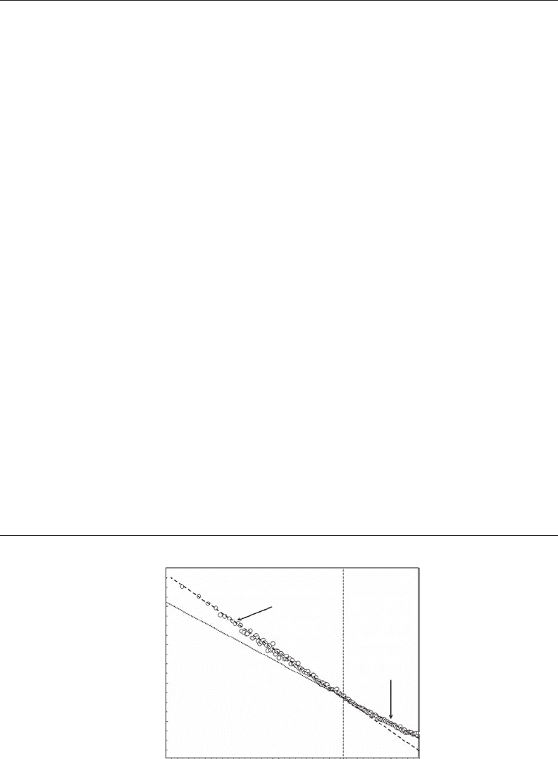
Samples of the double logarithmic power spectra for the studied time series together with their

best tting lines are given in Figure 4.10. The power spectra present a mixed behavior with two

scaling tendencies, the change of behavior of the power spectra occurring for frequencies

ranging

from 0.02 to 0.11 Hz (

0.06 0.03±

Hz,

x ±SD

), which are associated with characteristic time scales

ranging from about 9 to 54 seconds (

23.3 12.9±

sec,

x ±SD

). Within each data set, the transition

scales are very similar whatever the variables in question, as shown by the weak dispersion of the

estimates of the transition frequencies

(

=±0.005 0.001

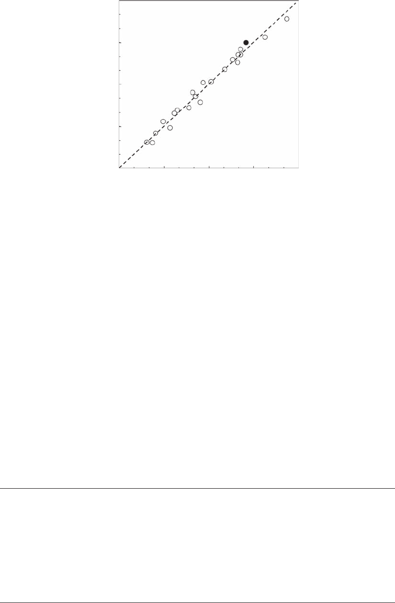
Those temporal transition scales can be associated with spatial scales using Taylor’s hypothesis

of frozen turbulence (Taylor 1938), which basically states that temporal and spatial averages

and

l, respectively, can be related by a constant velocity

V ,

lVt=⋅.

Then, using the mean tidal drift

observed during each eld experiment (Table 4.1), we estimate that the associated length scales

were ~12 meters (

12.1 1.6±

x ±SD

) for sampling experiments S1 to S21 and 24.6 meters for

sampling experiment S22. These length scales are close to the size of the ships used during the

sampling experiment, that is, 12.5 m and 24.9 m for N/O Sepia II and N/O Côte de la Manche,

respectively. These results thus conrm and generalize the results obtained by Seuront et al. (1996b)

from a single sampling experiment conducted at the end of March 1995 during a period of spring

tide (Table 4.2; Figure 4.11).

In order to interpret this change of behavior of the power spectra, remember that the measure-

ments were taken from a boat adrift in the channel. This means that for the high-frequency range

table 4.1

summary of the date, location, sampling Frequency f (hz), tide (m s

–1

), wind speed

(m s

–1

), and direction (°) for the 22 sampling experiments

code date latitude longitude f depth tidal current wind

speed direction speed direction

S1 March 30,1995

50°40900 l°31900

2 15.7 1.00 180 7 120

S2 November 29,1995

50°48956 1°29945

2 14.7 0.22 90 5 22

S3 January 19, 1996

50°52924 1°34993

1 7.6 1.12 0 6 230

S4 February 1, 1996

50°42973 1°27949

1 15.8 0.60 0 3 220

S5 February 22,1996

50°43909 l°32930

1 6.2 0.88 180 4 90

S6 March 28,1996

50°45956 1°33982

2 10.4 0.28 180 8 90

S7 April 26, 1996

50°55926 1°32964

2 16.8 0.45 90 3 170

S8 May 28, 1996

50°49993 1°32993

2 15.6 0.75 0 3 90

S9 June 3, 1996

50°49935 1°31962

2 16.1 1.50 0 6 130

S10 June 19, 1996

50°42942 1°2895I

2 10.5 1.01 180 1 260

S11 June 25, 1996

50°51921 1°29965

2 21.2 0.91 180 1 330

S12 September 4, 1996

50°40953 1°30963

2 5.9 0.99 180 5 310

S13 September 25, 1996

50°44973 l°33905

2 6.2 0.39 0 5 210

S14 September 25, 1996

50°44991 1°33919

2 11.2 0.39 0 5 210

S15 September 25, 1996

50°45939 1°33945

2 15.8 0.39 0 5 210

S16 October 2, 1996

50°42908 l°32990

2 6.6 0.69 180 1 100

S17 October 2, 1996

50°42908 l°32990

2 6.0 0.69 180 1 100

S18 October 2, 1996

50°42908 l°32990

2 6.2 0.69 180 4 40

S19 October 8, 1996

50°47979 l°33968

2 6.3 0.50 0 1 220

S20 December 5, 1996

50°45950 1°32985

2 6.6 0.30 0 2 190

S21 December 18, 1996

50°45946 1°32987

2 5.9 0.60 0 6 210

S22 April 2, 1998 50°45’00 l°33’50 2 6.0 0.60 0 2 100

2782.indb 114 9/11/09 12:08:34 PM

Self-Afﬁne Fractals 115

table 4.2

temporal and spatial transition scales between eulerian and lagrangian regimes

time series time (s)

time (s)

space (m)

* 12.30 12.70 12.30 12.70

S1 12.59 12.70 12.59 12.70

S2 53.70 54.00 11.81 11.88

S3 10.23 10.50 11.46 11.76

S4 21.38 21.00 12.83 12.60

S5 12.88 12.67 11.34 11.16

S6 44.67 44.00 12.51 12.32

S7 25.70 26.00 11.57 11.70

S8 16.22 16.50 12.16 12.38

S9 8.91 9.00 13.37 13.50

S10 12.30 12.00 12.43 12.12

S11 14.13 14.00 12.85 12.74

S12 12.30 12.50 12.18 12.38

S13 33.33 33.50 13.00 13.07

S14 30.90 31.00 12.05 12.09

S15 33.88 34.00 13.21 13.26

S16 18.62 19.00 12.85 13.11

S17 17.78 18.00 12.27 12.42

S18 19.50 20.00 13.45 13.80

S19 26.92 27.00 13.46 13.50

S20 40.74 41.00 12.22 12.30

S21 19.50 19.50 11.70 11.70

S22 44.68 44.50 24.58 24.48

Note: The association between temporal and spatial transition scales has been done via the Taylor’s hypothesis of frozen

turbulence.

Power spectra.

Structure functions.

Source: From Seuront et al. (1996b).

Log E ( f )

Log f

β ≈ 2

β ≈ 5/3

–1

–3

–4.5 –4.0 –3.5 –3.0 –2.5 –2.0 –1.5 –1.0 0.0–0.5

Figure 4.10 Power spectrum of temperature uctuations recorded in the inshore waters of the eastern

English Channel from a drifting boat 12.5 m long. Two scaling regimes with E( f ) ≈ f

−

and E( f ) ≈ f

−

5/3

respectively occur above and below a critical time scale t = 22 seconds. The high and low frequency regimes

correspond to Eulerian and Lagrangian regimes, respectively.

2782.indb 115 9/11/09 12:08:37 PM

116 Fractals and Multifractals in Ecology and Aquatic Science

of the measurements we can consider the boat as not moving, so the measurements correspond to

a xed-point procedure, that is, Eulerian sampling. This is conrmed by the slopes of the small-

scale temperature, salinity, and in vivo uorescence power spectra (Table 4.3), which were not

signicantly different (Kruskal-Wallis test,

P > 005.

) and cannot be statistically distinguished

from the theoretical spectral value

= 53/

(Binomial test,

p > 0.05) (Siegel and Castellan 1988)

expected in the case of an isotropic three-dimensional homogeneous turbulence (Obukhov 1949;

Corrsin 1951). Nevertheless, for each sampling experiment, an analysis of covariance (Zar 1996)

has been conducted for the slopes of the power spectra for temperature, salinity, and in vivo uo-

rescence. It is found that the chlorophyll a concentration exhibits highly signicant positive corre-

lation ( p = 0.01) with the F-statistic, used here as a measure of any signicant difference between

the slope of temperature, salinity, and uorescence power spectra for a given sampling experi-

ment. Subsequent multiple comparison procedures based on the Tukey test (Zar 1996) conducted

to determine which

was different from the others then conrmed and specied the previous

results. These analyses indicate that rejection of the null hypothesis was always due to

v a lu e s

for in vivo uorescence signicantly higher than those for temperature and salinity. On the con-

trary, light transmission power spectra (Table 4.3) appear signicantly smaller than the theoretical

0.12

0.09

0.06

0.03

0.00

0.00 0.03 0.06

eoretical Scale Breaking

Empirical Scale Breaking

0.09 0.12

Figure 4.11 Theoretical vs. empirical scale breakings (Hz) between Eulerian and Lagrangian scales.

Theoretical scale breaking has been estimated by multiplying the size of the boat used during the sampling

experiment by the mean tidal drift observed during each experiment. Empirical scale breaking has been esti-

mated as the mean transition scale from the power spectra of temperature, salinity, and in vivo uorescence.

The result obtained by Seuront et al. (1996b) is shown for comparison (black dot).

table 4.3

mean Values of the spectral exponent

ββ

estimated from time series of temperature,

salinity, In Vivo Fluorescence, and light transmission

temperature salinity Fluorescence transmission

E 1.70 (0.05) 1.72 (0.06) 1.69 (0.03) 1.31 (0.36)

L 2.03 (0.05) 2.03 (0.04) 1.03 (0.24) 1.02 (0.24)

Note: The numbers in parentheses are the standard deviations;

Eulerian (E; n = 22) and Lagrangian (L; n = 13) scales.

2782.indb 116 9/11/09 12:08:42 PM

Self-Afﬁne Fractals 117

=53/

value

(.).p < 005

Finally, one may also note here that analyses of covariance showed that

the 22 spectral exponents

were not all equal for each parameter, indicating potential differen-

tial spectral structures of the variables in question at the space-time scales of the whole sampling

experiment.

For frequencies smaller than the observed scale breakings, the inertia of the boat becomes neg-

ligible and the measurements are effectively taken following the ows, that is, in a Lagrangian

framework. One may note here that we had to average the original time series up to the Eulerian/

Lagrangian transition scale (Table 4.2) in order to be in the Lagrangian scales. In that way, our

characterization of the Lagrangian behavior of time series of temperature, salinity, light transmis-

sion, and in vivo uorescence is based on time series exhibiting at least 256 data points (that is, the

lower recommended bound for a data set to lead to reliable spectral analysis). In the following, we

then focused on 13 time series S1–S3, S5, S7, S9, S10–S12, S14, S19, and S21–S22. The previously

described transition is also conrmed by the similar scaling behaviors exhibited by temperature

and salinity time series (Table 4.3), which cannot be statistically distinguished from the theoreti-

cal slope

= 2

(Binomial test,

p > 005.)

expected in the case of purely passive scalars advected by

Lagrangian uid motions (Monin and Yaglom 1975). On the contrary, in vivo uorescence and light

transmission spectral exponents show very specic behaviors (Table 4.3) that cannot be statistically

distinguished (Wilcoxon-Mann-Whitney U-test, p > 0.05). Moreover, analyses of covariance con-

cluded that the 13 spectral exponents

were not all equal ( p < 0.05) for both light transmission and

uorescence power spectra.

4.2.2 dE T r E n d E d Fl u c T u a T i o n an a l y s i s

4.2.2.1 theory

Detrended uctuation analysis (DFA) is an elegant tool to quantify simply and reliably the corre-

lations found in both stationary and nonstationary data (Peng et al. 1992, 1993, 1994). Compared

to more traditional analyses used to estimate the degree of correlation in temporal signals, such

as power spectrum analysis (see Section 4.2.1), Hurst analysis (Section 4.2.5), and autocorrela-

tion analysis (Section 4.2.7), the advantage of the DFA method is that it can accurately quantify

the correlation property of signals masked by polynomial trends (Hu et al. 2001; Chen et al.

2002). Here, a temporal signal (note that the method described hereafter is also applicable to

a spatial signal x(l)), is integrated by computing for each t the accumulated departure from the

mean of the whole series:

Xt xi x

() [()]=−

∑

(4.29)

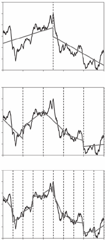
where N is the length of the data set. This integrated series is divided into nonoverlapping intervals

of length n. In each interval, a least-squares regression representing the trend in the interval is tted

to the data (Figure 4.12). The series X( t ) is then locally detrended by substracting the theoretical

values X

( t ) given by the regression. For a given interval length n, the characteristic size of uctua-

tions for this integrated and detrended series is calculated by:

Xt Xt

() [()()]=−

∑

(4.30)

This computation is repeated over all possible interval lengths. Note, however, that the width of

the regression windows ranged from six data points and to N/4 (Peng et al. 1994). The degree of

2782.indb 117 9/11/09 12:08:48 PM

118 Fractals and Multifractals in Ecology and Aquatic Science

correlation in the signal is nally quantied as:

F(l) ∝

DFA

(4.31)

where the exponent a is estimated as the slope of the linear trend of the log-log plot of F(l) versus l.

The use of a linear regression on the log-transformed data instead of nonlinear regression on the

raw data is recommended, as the residual error will be distributed as a quadratic and the mini-

mum error is not guaranteed. This is not the case with nonlinear regression (Seuront and Spilmont

2002).

As with power spectrum analysis, DFA allows the distinction between fGn and fBm signals; fGn

correspond to a

DFA

exponents ranging from 0 to 1, and fBm to exponents bounded between 1 and 2

X (t)X (t)X (t)

0 100 200 300 400 500

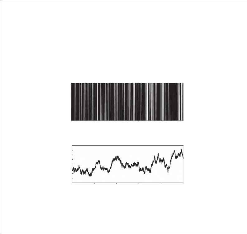
Figure 4.12 Three successive steps of the implementation of the detrended uctuation analysis (DFA). DFA

is applied to intervals of size (A), 100 (B), and 50 (C). The gray lines are the best least-squares t to the data

in each interval.

2782.indb 118 9/11/09 12:08:51 PM

Self-Afﬁne Fractals 119

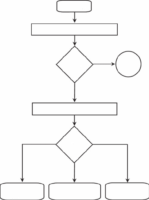
(Figure 4.13). Note that the correspondence between a and H is:

H = a

DFA

− 1 (4.32)

for fractional Brownian motions, and

H = a

DFA

(4.33)

for fractional Gaussian noises. The corresponding fractal dimensions, D

DFA

, are given by (Equation 4.9):

DFA

= 2 − H (4.34)

Note here that combining Equations (4.32) and (4.33) with Equations (4.13) and (4.14) leads to relate

the exponents a and b as a = ( b + 1)/2, and reciprocally b = 2 a − 1.

4.2.2.2 case study: assessing stress in interacting bird species

4.2.2.2.1 The Study Organisms

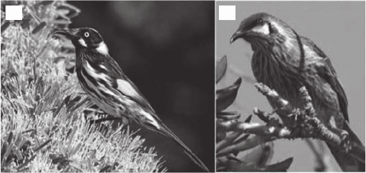
The New Holland honeyeater (Phylidonyris novaehollandiae; Figure 4.14A) and the red wattle-

bird (Anthochaera carunculata; Figure 4.14B) are Australian nectar-feeding passerines. The New

Holland honeyeater is a medium-sized (up to 18 cm) very active bird found throughout southern

Signal, Q(t)

Descriptive Statistics

DFA

Fractal Analysis to Estimate H

Signal Class

Stationary

Q(t) is fGn

Undeﬁned

Q(t) is fGn or fBm

Nonstationary

Q(t) is fBm

α > 1

α < 1

α = 1

Not

Fractal

Figure 4.13 Use of detrended uctuation analysis (DFA) to identify the class to which a data set belongs,

fractional Gaussian noise (fGn) or fractional Brownian motion (fBm), prior to further fractal analysis devoted

to estimate the Hurst exponent H, and the related fractal dimension.

2782.indb 119 9/11/09 12:08:54 PM

120 Fractals and Multifractals in Ecology and Aquatic Science

and southeastern Australia. It has a white iris, white facial tufts, and yellow markings on its wings

and tail feathers (Figure 4.14A). Although the New Holland honeyeater primarily feeds on nec-

tar, a large part of its diet may also consist of insects (Clarke and Clarke 1999; Kleindorfer et al.

2006). The red wattlebird is a larger (up to 35 cm) honeyeater and is considered a dominant hon-

eyeater species. It has red eyes, distinctive red wattles on either side of the neck (Figure 4.14B),

gray-brown body plumage, white streaks on the chest and belly, and a bright yellow patch on the

abdomen. Its range largely overlaps with that of the New Holland honeyeater but extends slightly

further inland, also occurring in southern and southeastern Australia. Red wattlebirds inhabit

coastal and woodland areas across a range of elevations. Both species thrive near habitation. Like

the New Holland honeyeater, red wattlebirds complement their diet with insects, berries, and

other fruits.

4.2.2.2.2 Experimental Procedures and Data Analysis

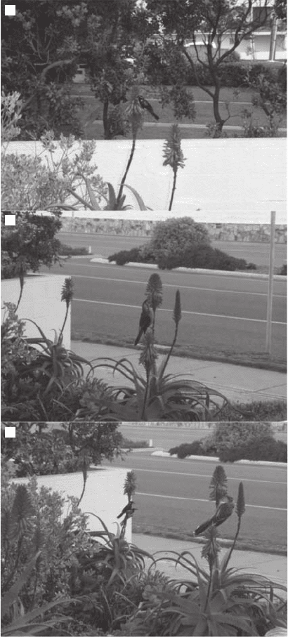
The behavior of New Holland honeyeaters and red wattlebirds was investigated when the birds were

eating the nectar of aloe owers separately (Figure 4.15A,B) and simultaneously (Figure 4.15C); the

objectives of this work were to investigate if their feeding behavior exhibited any long-term correla-

tion and if the presence of another species would affect the feeding behavior of a given species. The

behavior of those two species was recorded with a digital camera (DV Sony DCR-PC120E) at a rate

of 25 frame s

−1

on July 22, 2007, in West Beach, South Australia. The behaviors of New Holland

honeyeaters and red wattlebirds typically were very similar and consisted of either eating the nectar

with their beak in the ower or scanning their surroundings. The nature of the behavioral sequences

observed in the New Holland honeyeaters and the red wattlebirds was assessed through the con-

struction of a binary sequence z

(i) for each behavioral activity i taken from continuous observations

(Figure 4.16A,B). When a specic activity was observed, z

(i) = 1, and z

(i) = −1 otherwise. Here

(i) = 1 and z

(i) = −1 when the beak of either the New Holland honeyeater or the red wattlebird

was respectively inside and outside the ower. This generated binary sequences z

(i) taken at 0.04-

second time intervals t for each behavioral activity. Behavior sequence random walks w

( t ) were

subsequently obtained as

wt zi

() ()=

∑

(4.35)

where N is the number of behavioral observations. Equation (4.35) provides a graphical representa-

tion to calculate the degree of correlation in the behavioral time series (Figure 4.16C,D). Note the

clear difference between the behavioral z

( t ) and w

( t ) shown in Figure 4.16 and Figure 4.17 and

those obtained in case of a purely random process (Box 4.1).

Figure 4.14 The Australian nectar-feeding passerines (A) New Holland honeyeater (Phylidonyris novae-

hollandiae) and (B) red wattlebird (Anthochaera carunculata). (See color insert following page 80.)

2782.indb 120 9/11/09 12:08:57 PM

Self-Afﬁne Fractals 121

4.2.2.2.3 Results

Behavior sequence random walks w

( t ) obtained for New Holland honeyeaters (Figure 4.17A) and red

wattlebirds (Figure 4.17B) were visually clearly different, as was New Holland honeyeater behavior

in the absence (Figure 4.17B) and presence of red wattlebirds (Figure 4.17C). Specically, applying

Equations (4.30) and (4.31) to the behavior sequence random walks shown in Figure 4.17 leads to val-

ues of the exponent a

DFA

= 1.65 for New Holland honeyeaters and a

DFA

= 1.72 for red wattlebirds. The

values of a

DFA

obtained for the red wattlebird were not affected by the presence of the New Holland

honeyeater. In contrast, the exponent a

DFA

signicantly decreased down to a

DFA

= 1.48 for the New

Holland honeyeater in the presence of red wattlebirds.

4.2.2.2.4 Ecological Interpretation

The estimates of a

DFA

for the sequential behavior of the New Holland honeyeaters and the red wat-

tlebirds were consistently larger than 1, indicating that the behavior sequence random walks w

( t )

consistently belong to the class of fractional Brownian motions. Specically, the Hurst exponents

H estimated from Equation (4.32) lead to values higher than H = 0.5 for the New Holland hon-

eyeater (H = 0.65) and the red wattlebird (H = 0.72). Both species then exhibit a persistent behavior;

that is, a feeding bout is more likely to be followed by a feeding bout than by nonfeeding bout.

Box 4.1 PuRE RAnDoMnESS: CoIn FLIPPInG

The archetypical example of a purely random process is the ipping coin experiment in which

the probability of obtaining the obverse (heads) or the reverse (tails) is the same (that is, 0.5).

In addition, the probability of obtaining one event is totally independent of the previous event

(tails or heads); the coin-ipping process does not have memory.

The subsequent detrended uctuation analysis of

()

results in

DFA

=1.50,

hence

H = 0.50.

The sequential random walk

()

resulting from successive coin ipping is then a Brownian

motion; that is, no form of persistence

()H > 0.50

or antipersistence

()H < 0.50

exists in the

signal.

Figure 4.b1.1. Binary sequence obtained from 1000 iterations of a coin-ipping experiment, where

(i) = 1 for tails (black vertical lines, top panel) and z

(i) = −1 for heads (white vertical lines, top panel),

and the resulting sequential random walk

wt zi

() ()=

(bottom panel).

Sequence #

(i)

(t)

Sequence #

200 400 600 800 1000

–5

–15

200 400 600 800 1000

2782.indb 121 9/11/09 12:09:04 PM

122 Fractals and Multifractals in Ecology and Aquatic Science

In contrast, in the presence of the red wattlebird, the exponent H of the New Holland honeyeater

decreased to H = 0.48 and is nonsignicantly different from the special case H = 0.50 expected for

Brownian motion, which indicates no correlations in the behavior sequence w

( t ); in other words,

the probability of feeding bouts is independent of the probability of nonfeeding bouts. Those results

are consistent with previous behavioral studies using DFA to assess the health and stress from

binary behavioral sequences of wild chimpanzees (Alados and Huffman 2000) and captive chick-

ens (María et al. 2004). The exponents a

DFA

were consistently lower in sick chimpanzees than in

healthy ones, and decreased with chicken stress. The present results then suggest that the presence

Figure 4.15 The New Holland honeyeater (Phylidonyris novaehollandiae) and red wattlebird (Anthochaera

carunculata) foraging around aloe owers separately (A, B), and simultaneously (C).

2782.indb 122 9/11/09 12:09:06 PM

Self-Afﬁne Fractals 123

of the large red wattlebirds increases the level of stress in the New Holland honeyeaters, while the

signicantly higher a

DFA

observed for the red wattlebirds suggests an overall higher behavioral per-

sistence than might be related to their larger size. This is also consistent with other results based on

the use of cumulative frequency analyses and spectral analysis showing that the sequential behavior

of parasited Spanish ibex, Capra pyrenaica, which returned lower exponents in cumulative fre-

quency analyses (see Chapter 5) and spectral analysis than nonparasited ones (Alados et al. 1996).

A cumulative frequency analysis of the move duration observed in the marine zooplankton species

Centropages hamatus also showed a decrease in scaling exponent under conditions of naphtha-

lene contamination (Seuront and Leterme 2007). As a conclusion, detrended uctuation analysis of

sequential behavior in particular, and scaling analysis of sequential behavior in general, provide an

effective noninvasive method to record and evaluate the general state of health and related stress of

captive and wild animals.

Note that in their analysis of wild chimpanzee behavioral sequences, Alados and Huffman (2000)

seem to have mixed up the values of a

DFA

expected for fractional Brownian motions and fractional

Gaussian noises, as well as the concepts related to a

DFA

and H. They indeed claim that “a = 1 / 2

indicates no correlation in the sequence (white noise), and a ≠ 1/2 indicates long-range power law

correlations. If a exceeds 1/2, the sequence is persistent; if a < 1/2 the sequence is anti-persistent.”

However, as discussed in Section 4.2.2.1, this is only true for fGn in which case a

DFA

= H and is

bounded between 0 and 1. Over the 20 values of a

DFA

provided in their Table 3, 19 are greater than 1

and range between 1.114 and 1.436, suggesting that their random walks w

( t ) belong to the family of

fractional Brownian motions. As such, Equation (4.32) leads to a reinterpretation of the sequential

behavior of wild chimpanzees as being antipersistent (that is, a

DFA

< 1.5 and H < 0.5) and not per-

sistent as originally claimed (Alados and Huffman 2000). This stresses the critical need to identify

unambiguously the nature of a signal to be analyzed to ensure the results of the analysis are relevant

and meaningful.

(i)Z

(t)

(i)w

(t)

101 151 201

050 100 150 200

Sequence

050 100 150 200

151 101 151 201

–20

–40

–60

–80

–10

–40

–70

–100

–130

–160

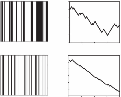
Figure 4.16 Examples of binary behavioral sequences z

(i) recorded for the New Holland honeyeater in

the (A) absence and (B) presence of the red wattlebird and respectively visualized as black and white vertical

lines for z

(i) = 1 (bird’s beak inside aloe ower) and z

( i ) = −1 (bird’s beak outside aloe ower). The binary

sequences z

(i) are subsequently used to build behavior sequence random walks w

( t ) as

wt zi

() (),=

w h e r e

N is the number of behavioral sequences.

2782.indb 123 9/11/09 12:09:09 PM