Seuront L. Fractals and Multifractals in Ecology and Aquatic Science
Подождите немного. Документ загружается.

94 Fractals and Multifractals in Ecology and Aquatic Science
each box of length d, the mean values x
i
(d ) and x
j
(d ) of the descriptor X(i, j) along longitudinal and
latitudinal transects are recorded and expressed, modifying Equation (3.34) as:
xk in
i
D
i
t
i
() ,,
δδ
==1
(3.85)
xk jn
j
D
j
tj
() ,,
δδ
==1
(3.86)
where k is a constant, n
i
and n
j
are the numbers of lines and columns of the Euclidean domain
supporting the descriptor X(i, j), and
D
t
i
and
D
t
j
the transect dimensions of the ith and jth lon-
gitudinal and latitudinal transects, respectively. Note that the transect dimensions
D
t
i
and
D
t
j
are conceptually similar to the cluster dimension introduced in Section 3.2.3.
The mean fractal dimensions of the latitudinal and longitudinal transects are given as:
D
n
D
t
i
t
i
n
ii
i
=
=
∑
1
1
(3.87)
D
n
D
t
j
t
j
n
jj
j
=
=
∑
1
1
(3.88)
The resulting one-dimensional transect dimension
D
t
ij,
of the surface is subsequently given as:
DDD
ttt
ij ij,
()=+
1
2
(3.89)
and the two-dimensional transect dimension of the surface is nally estimated as:
DD
tt
ij ij,,
=+1
(3.90)
Note that Equation (3.87) through Equation (3.89) are relevant only when the isotropy condition is
fully satised (see Section 7.2.2), and then requires an appropriate statistical test of homogeneity
between the n
i
and n
j
dimensions
D
t
i
an
D
t
j
; see Zar (1996).
3.2.9.2 contour dimension, D
co
This method is based on a conversion of a surface plot to a contour map, and using the dividers
method (see Section 3.2.1) to estimate the fractal dividers dimension D
d
i
of each of the n contours
(Figure 3.35). The contour dimension D
co
is directly expressed as:
D
n
D
co d
i
n
i
=+
=
∑
1
1
1
(3.91)
However, this method is implicitly highly dependent on the number of isolines used in the com-
putation of the fractal dimension D
co
. In particular, when applied to a topographic surface, the
consideration of more isolines should result in an increase of the resolved details and in subsequent
modications of the fractal dimension estimates.
2782.indb 94 9/11/09 12:07:27 PM
Self-Similar Fractals 95
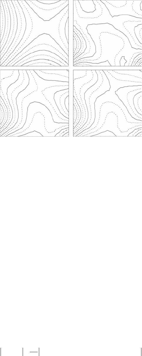
On the other hand, in the specic case of the two-dimensional distribution of a descriptor X(i, j), the
fractal dimension estimates returned by this method will be strongly inuenced by the interpolation pro-
cedure used to build the two-dimensional contour plots, which might themselves appear as being very dif-
ferent (Figure 3.36). As a consequence, any fractal dimension estimated using the contour method should
make explicit reference to the interpolation procedure used to build the two-dimensional contours.
3.2.9.3 geostatistical dimension, D
g
The geostatistical dimension D
g
is a two-dimensional generalization of the variogram dimension
introduced in Section 4.2.8 to self-similar patterns. The fractal dimension of a landscape surface is
based on the semivariance g (h) dened as (Huang and Turcotte 1989):
γ
()
()
[(,) (,)(,) (
()
h
Nh
XijXihjXij Xi
i
Nh
=−++ −
=
∑
1
4
1
2
,, )]
()
jh
j
Nh
+
=
∑
2
1
(3.92)
A
B
D
d
i
Chlorophyll (mg · m
–2
)
7.979
8.349
8.719
9.088
9.458
9.828
10.198
10.568
10.938
11.308
11.878
12.047
12.417
12.787
13.157
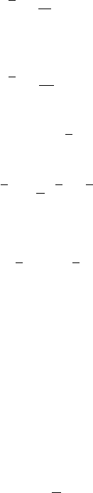
Figure 3.35 The contour dimension. Schematic illustration of the way to estimate (A) the two-dimensional
fractal dimension of a pattern from (B) the one-dimensional fractal dimensions of its n contours. The two-
dimensional fractal dimension is estimated as the mean of one-dimensional contour dimensions. The gray and
black broken lines indicate two successive steps of the divider method.
2782.indb 95 9/11/09 12:07:29 PM
96 Fractals and Multifractals in Ecology and Aquatic Science
where X(i + h, j) and X(i, j + h) are the values of the dependent variable X(i, j), that is, bacterioplank-
ton abundance, or microphytobenthos chlorophyll concentration in the above examples, at locations
separated by a distance h, and N(h) is the number of pairs of data points separated by the distance h.
The plot of g (h) as a function of h is referred to as a semivariogram, and the fractal dimension is
estimated from the slope m of the log-log plot of g (h) vs. h as:
D
g
= 3 − m/2 (3.93)
where D
g
is the geostatistical dimension.
3.2.9.4 elevation dimension, D
e
This method, based on the mean absolute elevation difference |Δ h| between two points separated
by a distance d, has been specically developed to estimate the fractal dimension of topographic
surfaces (Polidori et al. 1991). The related fractal dimension D
e
is given as:
||∆hk
D
e
=
−
δ
3
(3.94)
where k is a constant. Considering the two-dimensional distribution of a descriptor X(i, j), Equation
(3.94) is rewritten as:
||∆Xijk
D
e
(, )
δ
δ
=
−3
(3.95)
where k is a constant and |ΔX (i, j)
d
| is the mean absolute difference between the values of X(i, j)
separated by a distance d in the x-y plane and expressed as:
∆Xij
N
XijXij XijXij(, )((, )(,))((, )(,))
δ
δ
δδ
=−++ −+
1
(3.96)
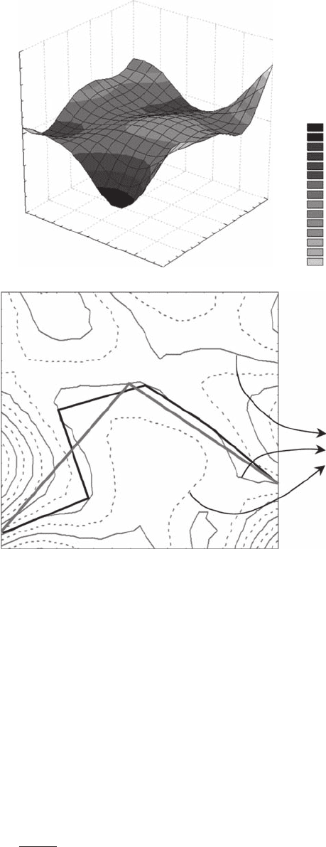
A
B
CD
D
co
= 1.05 D
co
= 1.35
D
co
= 1.30D
co
= 1.15
Figure 3.36 Illustration of the potential effects of the interpolation procedure used to build the two-dimen-
sional contour plots, that is, quadratic (A), mean square (B), negative exponential (C), and splines (D), on the
resulting contour dimensions.
2782.indb 96 9/11/09 12:07:33 PM
Self-Similar Fractals 97
Although the geostatistical and the elevation dimensions can provide a valuable estimate of the
two-dimensional fractal structure of a descriptor X(i, j)—for example, bacterioplankton abundance
or microphytobenthos biomass—it is straightforward to see that Equations (3.92) and (3.96) imply
different forms of spatial averaging. These two methods are then implicitly based on the stationarity
hypothesis discussed in Section 7.2.3 and cannot provide any information regarding potential differ-
ences in the local fractal structures. Such information is available using the transect and the contour
dimensions. The transect and the contour dimensions and the geostatistical and elevation dimen-
sions can be referred to as local fractal dimensions and global fractal dimensions, respectively.
2782.indb 97 9/11/09 12:07:34 PM
2782.indb 98 9/11/09 12:07:34 PM

99
4
Self-Affine Fractals
4.1 seVeral stePs toward selF-aFFinity
4.1.1 d
E F i n i T i o n s
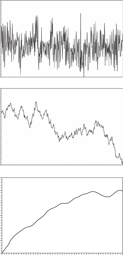
Consider, for example, a turbulent velocity component measured as a function of time at a single
point. As shown in Figure 4.1, it looks rough, like the boundary of a random fractal, but with the
difference that the two axes correspond to different physical quantities (velocity and time) that are
intrinsically different. Different units can be chosen for the two axes to make the trace look either
very steep or nearly smooth. Similarly, from a scalar eld in two dimensions, one can construct a
mountain-like structure in which the height at each point equals the magnitude of the local con-
centration (see Figure 3.33). Again, the height and the two spatial coordinates are intrinsically
different and independent, so that the mountain can be made to look jagged or relatively smooth
depending on the choice of units for the two quantities. In general, whenever different quantities
involved in such constructions scale differently, the notion of self-similarity contained in Equations
(3.1) through (3.3) will not be adequate; to describe these phenomena, one needs the more versatile
machinery of self-afnity.
An afne transformation is one that transforms a set S of points at positions
xxxx
D
E
=(, ,, )
12
into a new set d(S) with points at
δδδδ
() (, ,, )
xxxx
DD
EE
=
11 22
, where the scale ratios
(, ,, )
δδ δ
12
D
E
are all different. A bounded set S is self-afne when S is the union of N nonoverlapping subsets,
each of which is identical (under translations and rotations) to d(S). In other words, if a subset of a
pattern is similar to the whole under an afne transformation, the pattern is said to be self-afne.
In addition, S is statistically self-afne when S is the union of N distinct subsets, each of which is
identical in distribution to d(S). One cannot, however, dene fractal dimension using Equation (3.1)
through Equation (3.3) for even the simplest self-afne fractal curve. If one evaluates this dimen-
sion mechanically, pretending the curve in Figure 4.1 to be like a coastline, the value depends on
the expansion used for one quantity relative to the other. If, for example, the time scale is stretched
enough to render the signal to appear as a collection of smooth increments, it is intuitively clear
that the dimension (called the global dimension) will be unity. If, on the other hand, the ordinate
is stretched over a wide range of values, one can dene the usual fractal dimension according
to Equation (3.1). This is the so-called local dimension of the self-afne fractal. Although it has
been pointed out that more than one dimension is necessary to characterize self-afne fractals
(Mandelbrot 1986), and thus referring to the concept of multifractals studied more thoroughly here-
after (see Chapter 8), one must note that the fractal dimension for self-afne fractals is not as easily
dened as with self-similar ones.
4.1.2 Fr a c T i o n a l br o w n i a n mo T i o n
First, one needs to introduce the concept of fractional Brownian motion (fBm) (Mandelbrot and
Wallis 1969; Mandelbrot 1977, 1983), which can be thought of as a generalization of the so-
called concept of Brownian motion that played such an important role in both physics and math-
ematics. A fractional Brownian motion, B
H
(x), is a single valued function of one variable, x (that
2782.indb 99 9/11/09 12:07:37 PM
100 Fractals and Multifractals in Ecology and Aquatic Science
is, time or space) dened by its increments B
H
(x
i
) − B
H
(x
i−1
) that have a Gaussian distribution
with variance
|()()| ||Bx Bx kx x
Hi Hi ii
H
−=−
−−1
2
1
2
(4.1)
where k is a constant, the angle brackets “
〈〉
” denote ensemble averaging, and the parameter H,
0 < H < 1. Practically, Equation (4.1) means that its mean square increments depend only on the differ-
ence (t
i
− t
i−1
). In case of H = 0.5, Equation (4.1) recovers the Brownian motion where ΔB
2
= kΔt. More
formally, for any three time (x
i−1
, x
i
, and x
i+1
) such that x
i−1
< x
i
< x
i+1
, ΔB
1
= B
H
(x
i
) − B
H
(x
i−1
) is statisti-
cally independent of ΔB
2
= B
H
(x
i+1
) − B
H
(x
i
) for H = 0 .5 . This means that at every stage and at every
scale of Δt, all directions of displacement are equally likely. For H > 0.5 and H < 0.5, the increments
are positively and negatively correlated, respectively. More specically, if H > 0.5, the increments of
the displacement may be roughly thought of as overlapping each other, above time increments that
do not overlap. Such a process may be said to be positively correlated, or persistent, in the sense that
a particle moving in some direction at time t will tend to move in the same direction regardless of Δt.
Alternatively, if H < 0.5, the process is said to be negatively correlated, or antipersistent.
It can be seen that Equation (4.1) is qualitatively similar to a power law. Any change by a factor
of d in the scale t will change ΔB
H
by a factor of d
H
as:
∆=∆Bx kBx
H
H
H
() ()
δδ
22 2
(4.2)
where k is a constant. Practically, Equation (4.1) introduces a major difference to the self-similar
power law; see, for example, Equations (3.1) and (3.2). Indeed, a fractional Brownian trace requires
different scaling factors in the two coordinates (d for x, and d
H
for B
H
). Each value of x corresponds
to only one value of B
H
, while any value of B
H
may occur at multiple values of x. This specic non-
uniform scaling provides an additional denition to self-afnity.
4.1.3 di m E n s i o n o F sE l F -aF F i n E Fr a c T a l s
Consider a trace of B(x) covering a time span Δt = 1 and a vertical range B(x) = 1. B(x) is statistically
self-afne when t is scaled by d and B(x) is scaled by d
H
. Divide now the time span into N equal
intervals, each with Δt = 1 / N. Each of these intervals contains one portion of B(x) with vertical range
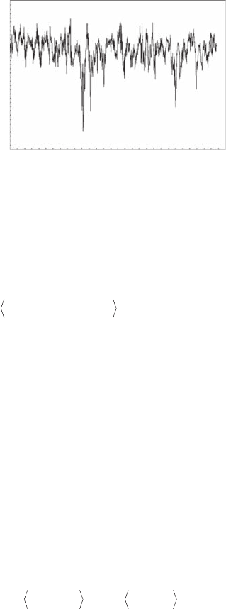
Turbulent Velocity (relative units)
3100
3050
3000
2950
2900
2800
2750
0 1000 2000 3000 4000 5000 6000
Time (s/100)
2850
Figure 4.1 A time series of microscale turbulent velocity uctuations, as an illustration of a self-afne
fractal.
2782.indb 100 9/11/09 12:07:41 PM
Self-Affine Fractals 101
ΔB = Δt
H
. Since 0 < H < 1, each of these new sections will have a large vertical and horizontal size
ratio and the occupied portion of each interval will be covered by ΔB/Δt = (1 /N
H
)/(1/N) = N/N
H
elements of size d
n
= 1 / N. The number of length elements required to cover the trace goes from 1
to N(d
n
) as:
NNNN
n
H
n
H
() //
δδ
=× =
−
1
2
(4.3)
Finally, comparing Equations (3.2) and (4.3) leads to the fractal dimension D
F
:
D
F
= 2 − H (4.4)
A Brownian motion will thus have a fractal dimension D
F
= 1.5.
Fractional Brownian motion, illustrated here in a one-dimensional framework, can be general-
ized to higher dimensions, namely to self-afne surface and volume. For instance, replacing the
single variable x by the coordinates (x, y) in a plane leads to considering the resulting fBm B
H
(x, y)
as the surface altitude at position (x, y). In analogy with Equation (4.1), the increments B
H
(x
i
, y
i
) −
B
H
(x
i−1
, y
i−1
) of B
H
(x, y) have a Gaussian distribution with variance:
|(,) (, )| [( )(BxyBxy kx xyy
HiiHii ii i
−=−+−
−− −11
2
1
2
ii
H
−1
2
)]
(4.5)
From Equation (4.4), the fractal dimension of a fractal landscape can be derived as:
D
F
= 3 − H (4.6)
Note that the intersection of a vertical plane with the surface B
H
(x, y)—that is, the altitude uctua-
tions of a mountain sheep following any straight path in the (x, y) plane—is a self-afne fractional
Brownian motion fully similar to those observed in Figure 4.2 with D
F
= 2 − H. Alternatively, the
intersection of a horizontal plane with the surface B
H
(x, y)—that is, the coastline of a mountain
lake—has a fractal dimension D
F
= 3 − H, but since the two coordinates x and y are equivalent, the
coastlines of B
H
(x, y) are self-similar, not self-afne. A fractal volume—that is, a fractal cloud—has
the fractal dimension:
D
F
= 4 − H (4.7)
Generally speaking, a self-afne fractional Brownian function,
Bx
H
(),
in a D
E
Euclidean space
satises:
|()()| ||Bx Bx kx x
Hi Hi ii
H
−=−
−−1
2
1
2
(4.8)
with
xxxx
D
E
=(, ,, ),
12
and its fractal dimension is written as:
D
F
= D
E
+ 1 − H (4.9)
Finally, the intersection of
Bx
H
()
with a D
E
-dimensional object form a self-similar fractal with
dimension D
F
= D
E
− H.
2782.indb 101 9/11/09 12:07:46 PM
102 Fractals and Multifractals in Ecology and Aquatic Science
4.1.4 1/f no i s E , sE l F -aF F i n i T y, a n d Fr a c T a l di m E n s i o n s
Self-afne functions have been dened (via fractional Brownian motion) as being a function of
a single variable x that can be regarded as either space or time, mainly because changes in space
have many of the same similarities at different scales as changes in time. However, unpredictable
changes of any quantity x( t ) varying in time t are known as noise. More specically, Montroll and
Badger (1974), Montroll and Shlesinger (1982), and West and Shlesinger (1990) have reported a
number of examples showing that when the spectral density E
Q
( f ) (that is, an estimate of the mean
square uctuations at frequency f, and consequently of the variations over a time scale of order 1/f )
Brownian Function Values
10
60
50
40
30
20
0
10
60
50
40
30
20
0
10
60
50
40
30
20
0
D
F
= 1.9
A
D
F
= 1.5
D
F
= 1.1
B
C
50 100 150 200 250 300 350 400 450 5000
50 100 150 200 250 300 350 400 450 5000
50 100 150 200 250 300 350 400 450 5000
Time (or space)
Figure 4.2 Self-afne fractional Brownian motion (fBm) characterized by different fractal dimensions.
Note that the case D
F
= 1.5 corresponds to the basic Brownian motion.
2782.indb 102 9/11/09 12:07:49 PM
Self-Affine Fractals 103
of certain data are presented on log-log plots, the data appear as a straight line over a certain range.
Beyond that range, the straight line assumes the shape of a curve according to an inverse power law
of the form
Ef f
Q
() /,≈1
β
where f is the frequency and b a positive exponent referred to as the spec-
tral exponent. In particular, the 1/f
b
law, referred to as scaling 1/f noise (Mandelbrot 1983), can serve
as a powerful tool to describe music, speech, and a wide variety of noise. For instance, studying dif-
ferent compositions such as the First Brandenburg Concerto and Scott Joplin rags, Voss and Clark
(1975, 1978) found that composition having a frequency generated by 1/f sources sounded pleasing,
while those generated by 1/f
2
sounded too correlated, and those sounds generated from white noise,
namely by 1/f
0
sources, sounded too random. The spectral density of 1/f noise thus varies with a
predictability between white noise (1/f
0
, no correlation in time) and Brownian motion (
1
2
/,f
no
variability between increments; see Section 4.1.2). More generally, the so-called 1/f noise has been
observed in a wide variety of phenomena in nature, ranging from earthquakes (Bak and Tang 1989;
Carlson and Langer 1989), turbulence (Gollub and Benson 1980), cosmology (Chen and Bak 1989),
relaxation in nonperiodic solids (Evangelou and Economou 1990), ionization of excited hydrogen
atoms (Jensen 1990), microcirculatory control of blood ow (Intaglieta and Breit 1991), and human
interbeat dynamics (Nunes Amaral et al. 1998; Ivanov et al. 1999) to complex systems involving a
large number of interacting subunits that display “free will,” such as city growth (Makse et al. 1995)
and economics (Mantegna and Stanley 1995). An illustration of different
1/f
noises, together with
the related power spectra, is given in Figure 4.3.
Both white noise (1/f
0
, no correlation in time) and Brownian motion (1/f
2
, no correlation between
increments) are well understood in terms of mathematical physics. On the other hand, the origin of
1/f
b
noise, which represents the most common type of noise found in nature, nevertheless remains
a mystery after almost a century of investigations. The universality of 1/f noise suggests that it does
not represent a consequence of particular physical interactions but instead is a general manifestation
of complex dynamical systems that have remarkably similar critical components, perhaps because
the “interaction parts” between the constituent subunits in such extremely complex systems domi-
nate the observed cooperative behavior more than the detailed properties of the subunits themselves
(Stanley 1995). From a mathematical point of view, this universality may be attributed to a very rich
random statistical ensemble that has typical congurations dominating over the usual mean values
(West and Shlesinger 1989).
4.1.5 Fr a c T i o n a l br o w n i a n mo T i o n , Fr a c T i o n a l ga u s s i a n no i s E , a n d Fr a c T a l an a l y s i s
Fractional Gaussian noise (fGn) represents another family of self-afne processes, dened as the
series of successive increments in an fBm. An fBm signal is nonstationary with stationary incre-
ments. The increments, y( t ) = x( t ) − x(t − 1), of a nonstationary fBm signal x( t ) yield a stationary fGn
signal and vice versa. Fractional Gaussian noise and fractional Brownian motion signals are then
interconvertible: When an fGn is cumulatively summed, the resultant series constitutes an fBm, and
when an fBm is differenced, the resultant constitutes an fGn. Each fBm is then related to a specic
fGn, and both are characterized by the same H exponent. These two processes, however, possess
fundamentally different properties: fBm is nonstationary with time-dependent variance, while fGn
is a stationary process with a constant mean and variance expected over time. Examples of fBm and
fGn corresponding to three values of H are presented in Figure 4.4. The H exponent can be assessed
from an fBm series as well as from the corresponding fGn, but because of the different properties
of these processes, the methods of estimation are necessarily different. The dichotomy between fGn
and fBm motivated a systematic evaluation of fractal analysis methods (Caccia et al. 1997; Cannon
et al. 1997; Eke et al. 2000, 2002) that showed that most methods gave acceptable estimates of the
Hurst exponent H when applied to a given class (fGn or fBm) but led to inconsistent results for
the other. The rst step in a fractal analysis is to identify the class to which the analyzed data set
belongs, fGn or fBm (Figure 4.5). The Hurst exponent H can subsequently be properly estimated,
using a method relevant for the identied class. The nature of 1/f
b
noises described can here be very
2782.indb 103 9/11/09 12:07:52 PM