Schulz M. Control Theory in Physics and Other Fields of Science: Concepts, Tools, and Applications
Подождите немного. Документ загружается.


3.2 Extensions and Applications 75
3.2.2 Inhomogeneous Linear Evolution Equations
It may be possible that the linear evolution equations have an inhomogeneous
structure
˙
Y = AY + Bw + F, (3.68)
where F (t) is an additional generalized force. This problem can be solved by
a transformation of the state vector Y → Y
= Y − θ, where θ satisfies the
equation
˙
θ = Aθ + F (3.69)
so that the new evolution equation for Y
˙
Y
= AY
+ Bw (3.70)
remains. Furthermore, the transformation modifies the original performance
functional (3.43)in
J[Y, w]=
1
2
T
0
dt [(Y
(t)+θ(t)) Q(t)(Y
(t)+θ(t)) + w(t)R(t)w(t)]
+(Y
(t)+θ(T )) S (Y
(t)+θ(T )) . (3.71)
This result suggests that the class of linear quadratic control problems with
inhomogeneous linear evolution equations can be mapped onto the class of
tracking problems.
3.2.3 Scalar Problems
A special class of linear quadratic problems concerns the evolution in a 1d-
dimensional phase space. In this case all vectors and matrices degenerate to
simple scalar values. Especially, the differential Ricatti equation is now given
by
˙
G +2AG −
B
2
R
G
2
+ Q = 0 with G(T )=Ω. (3.72)
This equation is the scalar Ricatti equation, originally introduced by J.F.
Ricatti (1676–1754). A general solution of (3.72) is unknown. But if a particu-
lar solution G
(0)
of (3.72) is available, the Ricatti equation can be transformed
by the map G → G
(0)
+ g into a Bernoulli equation
˙g +2
A −
B
2
R
G
(0)
g −
B
2
R
g
2
=0, (3.73)
which we can generally solve. This is helpful as far as we have an analytical
or numerical solution of (3.72) for a special initial condition.
We remark that some special elementary integrable solutions are available
[10, 11, 12]. Two simple checks should be done before one starts a numerical
solution [13]:

76 3 Linear Quadratic Problems
• If B
2
α
2
=2αβAR + β
2
QR for a suitable pair of constants (α, β) then α/β
is a special solution of the Ricatti equation and it can be transformed into
a Bernoulli equation.
• If (QR)
B − 2QRB
+4ABQR = 0, the general solution reads
G(t)=
&
QR
B
2
tanh
t
0
QR
−1
|B|
dτ + C
. (3.74)
An instructive example of a scalar problem is the temperature control in
a homogeneous thermostat. The temperature follows the simple law
˙
ϑ = −κϑ + u, (3.75)
where ϑ is the temperature difference between the system and its environ-
ment, u is the external changeable heating rate and κ is the effective heat
conductivity. A possible optimal control is a certain stationary state given by
u
∗
= κϑ
∗
. Uncertainties in preparation of the initial state lead to a possible
initial deviation Y (0) = ϑ(0) − ϑ
∗
(0), which should be gradually suppressed
during the time interval [0,T] by a slightly changed control u = u
∗
+ w.Thus,
we have the linear evolution equation
˙
Y = −κY + w, i.e., A = −κ and B =1.
A progressive control means that the accuracy of the current temperature with
respect to the desired value ϑ
∗
should increase with increasing time. This can
be modeled by Q = αt/T , R =1,andΩ = 0. We obtain the Ricatti equation
˙
G − 2κG − G
2
+
αt
T
= 0 with G(T )=0. (3.76)
The solution is a rational expression of Ayri functions
G(t)=
'κA (x)+A
(x) − C'κB(x) − CB
(x)
A(x) − CB(x)
(3.77)
with A and B the Ayri-A and the Ayri-B function, 'κ = κ(T/α)
1/3
and x =
'κ
2
+(α/T )
1/3
t. The boundary condition defines the constant C
C =
'κA('κ
2
+ α
1/3
T
2/3
)+A
('κ
2
+ α
1/3
T
2/3
)
'κB('κ
2
+ α
1/3
T
2/3
)+B
('κ
2
+ α
1/3
T
2/3
)
. (3.78)
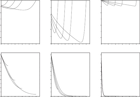
In order to understand the corresponding control law w
∗
= −GY
∗
and the op-
timal relaxation behavior of the temperature difference to the nominal state,
see Fig. 3.5, we must be aware that the performance integral initially sup-
presses a strong heating or cooling. In other words, a very fast reaction on an
initial disturbance cannot be expected. The first stage of the control regime is
dominated by a natural relaxation following approximately
˙
Y = −κY because
the contributions of the temperature deviations, QY
2
∼ tY
2
, to the perfor-
mance are initially small in comparison to the contributions of the control
function Rw
2
. The dominance of this mechanism increases with increasing
heat conductivity κ. The subsequent stage is mainly the result of the con-
trol via (3.77). We remark that the final convergence of G(t) to zero is a
3.3 The Optimal Regulator 77
012345
-3
-2
-1
0
w
*
012345
0,0
0,2
0,4
0,6
0,8
1,0
Y
*
012345
-3
-2
-1
0
012345
-3
-2
-1
0
012345
0,0
0,2
0,4
0,6
0,8
1,0
012345
0,0
0,2
0,4
0,6
0,8
1,0
ttt
Fig. 3.5. Scalar thermostat: optimal control functions w
∗
(top) and optimal tem-
perature relaxation Y
∗
(bottom) for different time horizons (T =1,2,3,and5.The
initial deviation from the nominal temperature is Y (0) = 1. The parameters are
κ =0,α =1(left), κ =0,α =10(center )andκ =10,α =10(right)
consequence of the corresponding boundary condition. The consideration of
a nonvanishing end point contribution to the performance allows also other
functional structures.
3.3 The Optimal Regulator
3.3.1 Algebraic Ricatti Equation
A linear quadratic problem with an infinite time horizon and with both the
parameters of the linear system and the parameters of the performance func-
tional being time-invariant is called a linear regulator problem [14]. Obvi-
ously, the resulting problem is a special case of the previously discussed linear
quadratic problems. The independence of the system parameters on time of-
fers a substantial simplification of the required mathematical calculus. Hence,
optimal regulator problems are well established in different scientific fields
and commercial applications [7, 15].
The mathematical formulation of the optimal regulator problem starts
from the performance functional with the infinitely large control horizon

78 3 Linear Quadratic Problems
J
0
[Y,w]=
1
2
∞
0
dt [Y (t)QY (t)+w(t)Rw(t)] → inf (3.79)
to be minimized and the linear evolution equations (3.41) with constant co-
efficients
˙
Y (t)=AY (t)+Bw(t) . (3.80)
By no means can the extension of a linear quadratic problem with a finite
horizon to the corresponding problem with an infinitely large horizon be inter-
preted as a special limit case. The lack of a well-defined upper border requires
also the lack of an endpoint contribution. To overcome these problems, we
consider firstly a general performance
J[Y, w,t
0
,T]=
1
2
T
0
dt [Y (t)QY (t)+w(t)Rw(t)] +
1
2
Y (T )ΩY (T ) (3.81)
with finite start and end points t
0
and T instead of functional (3.79). We
may follow the same way as in Sect. 3.1.4 in order to obtain the control
law (3.55), the evolution equations for the optimum trajectory (3.56), and
the differential Ricatti equation (3.53). The value of the performance at the
optimum trajectory using (3.55) becomes
J
∗
= J[Y
∗
,w
∗
,t
0
,T]=
1
2
T
t
0
dt [Y
∗
QY
∗
+ w
∗
Rw
∗
]+
1
2
Y (T )ΩY (T )
=
1
2
T
t
0
dtY
∗
Q + GBR
−1
B
T
G
Y
∗
+
1
2
Y (T )ΩY (T ) . (3.82)
From here, we obtain with (3.53) and (3.56)
J
∗
=
1
2
T
t
0
dtY
∗
−
˙
G − A
T
G − GA +2GBR
−1
B
T
G
Y
∗
+
1
2
Y (T )ΩY (T )
= −
1
2
T
t
0
dt
Y
∗
˙
GY
∗
+
˙
Y
∗
GY
∗
+ Y
∗
G
˙
Y
∗
+
1
2
Y (T )ΩY (T )
= −
1
2
T
t
0
dt
d
dt
[Y
∗
GY
∗
]+
1
2
Y (T )ΩY (T )

3.3 The Optimal Regulator 79
=
1
2
Y
∗
(t
0
)G(t
0
)Y
∗
(t
0
) , (3.83)
where the last step follows from the initial condition (3.54). We remark that
this result is valid also for the general linear quadratic problem with time-
dependent matrices. We need (3.54) for the application of a time-symmetry
argument. The performance of the optimal regulator may be written as
J
0
[Y
∗
,w
∗
]=J[Y
∗
,w
∗
, 0, ∞] . (3.84)
Since the performance of the optimal regulator is invariant against a transla-
tion in time, we have
J
0
[Y
∗
,w
∗
]=J[Y
∗
,w
∗
, 0, ∞]=J[Y
∗
,w
∗
,τ,∞] (3.85)
for all initial times τ if uniform initial conditions, Y (τ)=Y
0
, are considered.
Thus we obtain from (3.83) the relation
Y
∗
0
G(τ)Y
∗
0
=const for −∞<τ<∞ . (3.86)
Hence, we conclude that the transformation matrix G is time-independent.
This requires that the differential Ricatti equation (3.53) degenerates to a
so-called algebraic Ricatti equation [6]
A
T
G + GA − GBR
−1
B
T
G + Q =0, (3.87)
and the optimal control as well as the optimal trajectory is described by
(3.55) and (3.56) with completely time-independent coefficients. Therefore,
the optimal regular can be also interpreted as the mathematical realization of
a static feedback strategy.
3.3.2 Stability of Optimal Regulators
If the algebraic Ricatti equation is solved, the dynamics of an optimal reg-
ulator is completely defined by the control law (3.55) and the dynamics of
the state of the system (3.41). These both equations lead to the equation of
motion of the optimal trajectory (3.56). An initially disturbed system should
converge to its nominal state for sufficiently long times, i.e., we expect Y
∗
→ 0
for t →∞. This behavior has comprehensive consequences. If we justify a
regulator in such a manner that (3.55) holds, the initial deviation as well as
any later spontaneous appearing perturbation decreases gradually. The neces-
sary condition for this intrinsic stability of the regulator is that the evolution
equation of the optimal trajectory (3.56) is stable. That means the so-called
transfer matrix D of the linear differential equation system
˙
Y
∗
=
A − BR
−1
B
T
G
Y
∗
= DY
∗
(3.88)
must be positive definite.
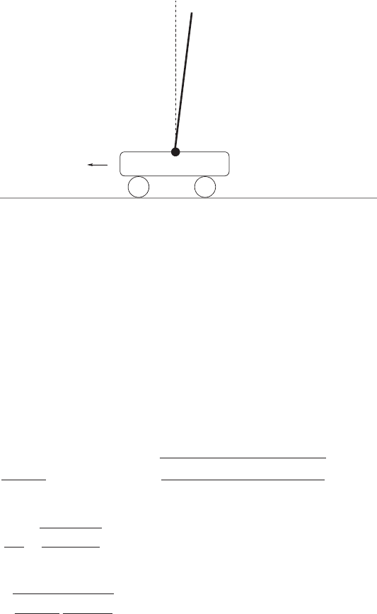
Let us study the inverted, frictionless pendulum as an instructive example.
The pendulum consists of a cart of mass M and a homogeneous rod of mass
80 3 Linear Quadratic Problems
F
J,m,l
ϑ,ϑ
.
M
x,x
.
Fig. 3.6. The inverted pendulum problem
m, inertia J and length 2l hinged on the cart (Fig. 3.6). The cart may move
frictionless under the external control force F along a straight line. Denoting
with ϑ the angle between the rod and the vertical axis and with x the position
of the cart, the equations of motion are given by
(M + m)¨x = ml(
˙
ϑ
2
sin ϑ −
¨
ϑ cos ϑ)+F (3.89)
(J + ml
2
)
¨
ϑ = mgl sin ϑ − ml¨x cos ϑ. (3.90)
The stationary but instable solution of this problem,
˙
ϑ
∗
=˙x
∗
= x
∗
= F
∗
=0
and x
∗
=const., may be our optimum solution. Now, we are interested in
the control of small perturbations. To this aim we introduce the dimensionless
quantities
y =
M + m
ml
(x − x
∗
),τ=
(
m(M + m)gl
(J + ml
2
)(M + m) − m
2
l
2
t, (3.91)
and
w =
F
mg
&
Jl
−2
+ m
M + m
, (3.92)
and the system parameter
ε =
&
M + m
m
J + ml
2
ml
2
. (3.93)
Thus, the linearized equations of motion are now ¨x = −ϑ+wε and
¨
ϑ = ϑ−w/ε.
This leads us to the state vector Y =(y, v, ϑ, ω) with v =˙y and ω =
˙
ϑ.The
control has only one component, namely, w. Hence, we get the matrices
A =
0100
00−10
0001
0010
and B =
0
ε
0
−ε
−1
. (3.94)
3.4 Control of Linear Oscillations and Relaxations 81
The matrix A is unstable, i.e., there exists some positive eigenvalues. Although
this example seems to be very simple, a numerical solution [16] of the alge-
braic Ricatti equation is required for a reasonable structure of the quadratic
performance functional. The main problem is that the nonlinear Ricatti equa-
tion has usually more than one real solution. However, the criterion to decide
which solution is reasonable follows from the eigenvalues of the transfer matrix
D = A − BR
−1
B
T
G.
Inverted pendulum systems are classical control test rigs for verification
and practice of different control methods with wide ranging applications from
chemical engineering to robotics [17]. Of course, the applicability of the linear
regulator concept is restricted to small deviations from the nominal behavior.
It is a typical feature of linear optimal regulators that they can control the un-
derlying system only in a sufficiently close neighborhood of the equilibrium or
of another nominal state. However, the inverted pendulum or several modifi-
cations [18, 19], e.g., the rotational inverted pendulum, the two-stage inverted
pendulum, the triple-stage inverted pendulum or more general a multi-link-
pendulum, are also popular candidates for the check of several nonlinear con-
trol methods. However, the investigation of such problems in beyond the scope
of this book. For more information, we refer the reader to the comprehensive
literature [20, 21, 22, 23, 24, 25].
In principle, one can also invert the optimal regulator problem, i.e., we ask
for the performance which makes a certain controller to an optimum regulator.
The first step, of course, is now the creation of a regulator as an abstract or
real technological device. We assume that the regulator stabilizes the system.
This is not at all a trivial task, but this problem concerns the wide field
of modern engineering [1, 26, 27, 28, 29]. The knowledge of the regulator is
equivalent to the knowledge of the transfer matrix D =
A − BR
−1
B
T
G
Y
∗
.
The remaining problem consists now in finding the performance index to which
the control law of the control instrument is optimal. This problem makes sense
because the structure of Q allows us to determine the weight of the degrees
of freedom involved in the control process [30].
3.4 Control of Linear Oscillations and Relaxations
3.4.1 Integral Representation of State Dynamics
Oscillations
Oscillations are a very frequently observed type of movement. In princi-
ple, most physical models with a well-defined ground state can be approx-
imated by the so-called harmonic limit. This is, roughly spoken, the expan-
sion of the potential of the system in terms of the phase space coordinates
X = {X
1
,X
2
,...,X
N
} up to the second-order around the ground state or

82 3 Linear Quadratic Problems
equilibrium state
4
. This physically pronounced state can be interpreted as the
nominal state of a possible control theory. Without any restriction we may
identify the origin of the coordinate system with the ground state, X
∗
=0.
This expansion leads to a linear system of second-order differential equations
¨
X
α
+
N
β=1
Ω
αβ
X
β
=0 for α =1,...,N (3.95)
or in a more compact notation
¨
X +ΩX = 0 with the frequency matrix
5
Ω.Of
course, this linearization is an idealization of the real object. However, the lin-
earized motion was thoroughly studied because of its wide applications. The
harmonic theory is a sufficient and suitable approximation in many scientific
fields, e.g., molecular physics and solid state physics or engineering. The in-
fluence of external forces f
i
α
requires the consideration of an inhomogeneous
term in (3.95). Thus, this equation can be extended to a more generalized
case
¨
X
α
+
N
β=1
Ω
αβ
X
β
= f
α
. (3.96)
The force f = {f
1
,f
2
,...,f
N
} can be interpreted as a superposition of driving
forces from external, but noncontrollable, sources ψ
α
(t) acting on each de-
gree of freedom α and the contributions of N
possible control functions
u = {u
1
,u
2
,...,u
N
} linearly coupled with the equations of motion
f
α
(t)=ψ
α
(t)+
N
β=1
B
αβ
u
β
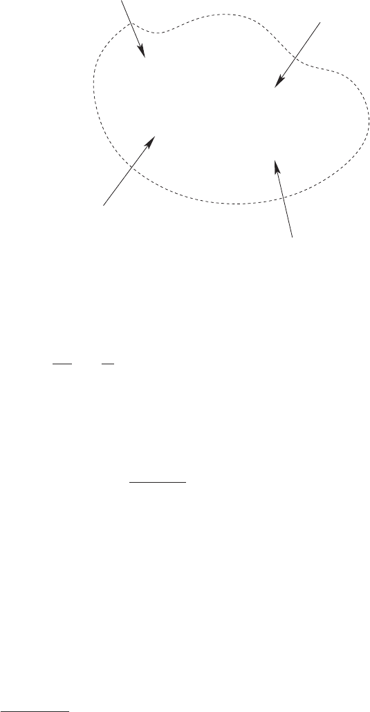
, (3.97)
where B is a matrix of type N ×N
with usually time-independent coefficients
(Fig. 3.7). In principal, system (3.96) can be extended to the generalized
system of linear differential equations
'
DX(t)=
+
Mf(t) (3.98)
with the differential operators
6
'
D =
n
k=1
a
k
d
k
dt
k
and
+
M =
n
k=1
b
k
d
k
dt
k
(3.99)
4
Or another sufficiently strong pronounced stationary state.
5
The frequency matrix is sometimes also denoted as the dynamical matrix.
6
Of course, we may reduce the higher derivatives to first-order derivatives but
this requires an extension of the phase space by velocities, accelerations, etc.
This prolongation method is the standard procedure discussed in the previous
chapters. However, in the present case such an extension of the phase space is not
desirable.
3.4 Control of Linear Oscillations and Relaxations 83
u
ψ
X
u
ψ
Fig. 3.7. External driving forces and control forces
The time-independent coefficients
7
a
k
and b
k
are matrices of the order N ×N .
For instance, a vibrational system with the linear Newtonian friction has the
operator
'
D =
d
2
dt
2
+ Λ
d
dt
+ Ω (3.100)
where the matrix Λ contains the friction coefficients. Equations of type (3.98)
can be formally solved. The result is a superposition of a solution with zero
external forces considering the initial state and a solution with a zero initial
state considering the external forces
X(t)=
n
k=1
H
k
(t)
d
k−1
X(t)
dt
k−1
t=0
+
t
0
H(t − τ)f(τ )dτ . (3.101)
The functions H
k
(t)andH(t) are called the response functions of the system.
These quantities are straightforwardly obtainable for example by application
of the Laplace transform
A(p)=
∞
0
dt exp {−pt}A(t) , (3.102)
which especially yields a polynomial representation of the differential opera-
tors
D(p)=
n
k=1
a
k
p
k
and M(p)=
n
k=1
b
k
p
k
. (3.103)
7
A more generalized theory can be obtained for time-dependent coefficients. For
the sake of simplicity we focus here only on constant coefficients.
84 3 Linear Quadratic Problems
From here we conclude that the Laplace transformed response functions are
simple algebraic ratios of two polynomials, e.g., H (p)=D(p)
−1
M(p).
Relaxation Processes
Obviously, (3.101) can be extended to all processes following generalized ki-
netic equations of the type
'
DX(t)+
t
0
K(t − τ )X(τ)dτ =
+
Mf(t) (3.104)
with a suitable memory kernel K(t). Physically, the convolution term in
(3.104) can be interpreted as a generalized friction indicating the hidden inter-
action of the relevant degrees of freedom of the system, collected in the state
vector X, and other degrees of freedom constituting a thermodynamic bath.
The causality of real physical processes requires always the upper limit t of
the integral. A general difference between (3.104) and the time-local equation
(3.98) is that the latter may be transformed always in a type of structure, but
a time-local representation of (3.104) cannot be obtained with the exception
of special cases. However, the integral representation of the solution of (3.104)
is again (3.101) with the exception that the Laplace transform of the response
function H(t) is now given by
H(p)=[D(p)+K(p)]
−1
M(p) . (3.105)
Evolution equation with memory terms are very popular in several fields of
modern physics, for example, condensed matter science, hydrodynamics, and
the theory of complex systems. The processes underlying the dynamics of
glasses [32, 33, 34] or the folding of proteins [35] are typical examples with
a pronounced memory. In particular, we can observe a stretched exponential
decay
K(t) ∼ exp {−λt
γ
} and γ<1 (3.106)
close to the glass transition of supercooled liquids [31, 36, 37].
The memory kernel can be determined by several theoretical and experi-
mental methods. Well established theoretical concepts are perturbation tech-
niques in the framework of the linear response theory [38, 40] or the calculus
of Green’s functions [39], or mode-coupling approaches [31, 33, 36], while var-
ious dielectric [42] and mechanical [41] methods as well as x-ray or neutron
scattering [43] are available for the experimental detection of memory effects.
Fractional Derivations and Integrals
A very compact representation of a special class of memory kernels is provided
by the fractional calculus [44]. Under certain conditions fractional integrals