Roy K.K. Potential theory in applied geophysics
Подождите немного. Документ загружается.

15.9 Integral Equation Method 529
unknown function to be determined. r and r
0
are respectively ‘the distances
of the points of observation and the source from the origin. If the Green’s
function is singular in a region of integration, then the equation is a singular
integral equation otherwise it is non-singular and continuous function. If the
equation can be solved for a certain value of λ, then the problem is said to be
an eigen value problem. In general it is easier to handle the integral equation
of the second kind. The most important component regarding the solutions of
the integral equation is the solution of these Green’s functions. Since Green’s
function appears under the integral equation, the integrals are solved using
numerical methods, viz. Gauss quadrature, Simpson’s rule, Weddles rule etc.
For simpler cases analytical solution of the integral is possible. In the case of
a discretized domain in IE, each element of the matrix equations becomes an
integral containing Green’s function. In integral equation method, distortion
in the field due to anomaly causing body are of interest. The anomaly causing
body of contrasting physical property in a half space or a layered half space is
replaced by the scattering current while formulation of the problem. In IEM,
these scattering currents are of interest to geophysicists. Therefore, the volume
of integration is r estricted to the anomaly causing b ody. As a result the size
of the matrix in formulation of an integral equation is considerably smaller
in comparison to th ose encountered while formulating the problems using
finite difference and finite element methods. Both FDM and FEM are differ-
ential equation based methods and entire spa ce outside the target body are
taken into consideration in the discretized domain. As a result IEM becomes
a very powerful tool for solving three dimensional boundary value problems.
In IEM, the matrices ar e solid but of much smaller size. In FDM and FEM,
the matrices are sparse but of large dimension. For modeling subsurface tar-
get body of complicated geometry, FDM and FEM have slight edge over IEM
with the gradual advancement in computation facilities. Mathematics may
become quite tougher in IEM in comparison to what we face for handling
FDM and FEM problems. FDM is well known for its inherent simplicity.
In electromagnetic boundary value problems, both scalar and tensor Green’s
function appear in the solution. Tensor Green’s function are known as dyadic
Green’s functions having 9 components. Therefore, the integral equation is
changed to matrix equation and these equations are solved using the method
of moments by judicious choice of the basis function and weighting function.
Green’s function becomes a tensor because the direction of the source dip ole
and the observation dipoles are in the different directions. Since the behaviours
of the dyadics is similar to that of a 3 ×3 tensor having nine components, the
dyadic Green’s function are termed as tensor Green’s function.
15.9.2 Formulation of an Electromagnetic Boundary
Value Pro blem
This subject is developed by Hohmann (1971, 1975, 1983, 1988), Wanna-
maker (1984a, 1984b, 1991), Meyer (1976), Weidelt (1975), Raichi (1975),
530 15 Numerical Methods in Potential Theory
Newman et al (1986), Newman et al (1987), Ting and Hohmann (1981). San-
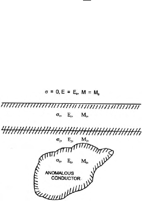
filipo and Hohmann (1985) and Sanfilipo et al (1985 Fig. (15.23) shows the
geometry of the problem. An anomalous b ody with a contrast in electrical
conductivity from the rest of the layered half space is assumed. The problem
is to determine the electrical and magnetic field due to the anomaly causing
body by replacing it with the scattering currents. These scattering currents
are in excess of conduction and displacement currents. These scattering cur-
rents are assumed in an otherwise homogeneous and isotropic layered half
space. Scattering current flows only through the conductivity inhomogeneity.
Computation of the anomalous fields is restricted to the volume occupied by
the target. Both primary and scattered secondary fields are harmonic fields.
In Maxwell’s equation
∇×
H=
J+
∂
D
∂t
, (15.220)
J is divided into two parts, i.e.,
J=
J
c
+
J
s
where
J
c
is the conduction current
because for most of the geo physical problems, displacement cur rent is negli-
gible. Displacement current becomes s ignificant in megahertz and gigahertz
range. J
c
is connected with the scalar conductivity σ.J
s
is the source current
which flows through the host rock. The first step in this scattering problem
is to replace the inhomogeneity by
J
s
.ThisJ
s
is the current density due to
the flow of current through the inhomogeneity. The electrical conductivity
of the anomalous region is σ
s
. The total electric field are field due to half
space without any inhomogeneity and that due to scattering current which is
superimposed over the conduction current. Therefore
Fig. 15.23. An anomalous conductor in a layered half space (Mayer 1976)
15.9 Integral Equation Method 531
E=
E
s
(r) +
E
i
(r). (15.221)
E
i
(r) is the electric field, that would exist at the field point or observation
point, in the absence of the anomalous body.
E
s
(r) is the scattered field at
r due to anomaly causing body.
E
s
(r) is a function of
J
s
whichexistsinthe
entire anomalous region. The relationship can be written as
E
s
(r) =
v
a
→
G(r,r
0
)
J
s
(r
0
)dv
0
(15.222)
Morse and Feshback (1953), Tai (1971), Hohman (1971), Van Bladel (1968),
Eskola (1992). Here v
a
is the anomalous volume for integration, r
0
is the
potential vector for the source point.
→
G(r,r
0
) is the tensor Green’s function,
because the direction of the field may or may not be in the same direction as
the current elements in the medium.
→
G(r,r
0
) is the scattered electric field at
r due to unit current density at r
0
.
E
s
(r) have some contribution due to the
magnetic current also. Since f ree space magnetic permeability µ
0
is assumed
for the entire half space with no contrast anywhere, therefore the magnetic
current is absent and is not included in the solution.
J
s
, the anomalous current
density is just the conduction current density in the anomalous body minus
the conduction current in the surrounding host rock. Therefore
J
s
(r
0
)=(σ
E
s
− σ
E
2
)
E
s
(r
0
) (15.223)
where σ
E
s
and σ
E
2
are the anomalous and true electrical conductivity in
the anomalous zone neglecting displacement current. Therefore we can write
(15.222) as
E
s
(r) =
v
a
→
G(r,r
0
)(σ
s
− σ
2
)
E(r
0
)dv
0
. (15.224)
Assuming σ
s
and σ
2
to be constant, (σ
s
−σ
2
) can b e taken out of the sign of
integration. Equation (15.224) can be rewritten in the form
E
s
(r) = (σ
s
− σ
2
)
v
a
→
G(r,r
0
)E(r
0
)dv
0
. (15.225)
Using (15.221), we can write
E(r) =
E
i
(r) + (σ
s
− σ
2
)
v
a
G(r,r
0
)
E(r
0
)dv
0
. (15.226)
Equation (15.226) is the vector Fredhom’s integral equation of the second kind.
E
i
(r), the electric field induced in the free space can be computed.
→
G(r,r
0
),
532 15 Numerical Methods in Potential Theory
the Green’s tensor, which depends upon the geometry of the problem, can be
calculated (Hohmann, 1975, Weidelt, 1975, Raichi, 1975, Wannamaker 1984,
Meyer, 1976). Equation (15.198) is used to calculate
E
i
(r). Equation (15.197)
is used to calculate
E
s
(r). Method of moments (Harrington, 1968) can be
based for solving (15.226) by proper choice of basis function and weighting
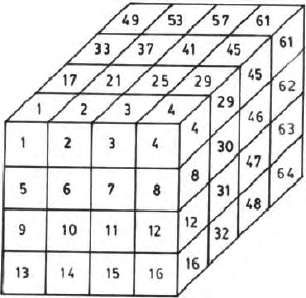
functions (Hohmann 1988). Volume V
a
of the anomalous conductor is divided
into N smaller volumes (Fig. 15.24.).
The electrical field within each of the smaller volumes are assumed to be
constant. The integral equation at the centre of each of these smaller cubical
volumes (Fig. 15.24) is
E
m
=
E
m
i
+
N
n=1
(σ
s
− σ
2
)
v
a
→
G(r,r
0
)
E
n
dv
0
. (15.227)
where
E
m
is the electric field of the centre of the mth cell. r
m
is the position
vector for the mth cell. It is the distance of the centre of the mth cell from
the origin.
Since
E
n
, the electric field in the nth cell (Fig. 15.25) is assumed to be
constant throughout the anomalous conductor,
E
n
can be taken outside the
sign of integration. Therefore (15.227) can be written as
E
m
=
E
m
i
+
N
n
(σ
s
− σ
2
)
v
a
→
G(r
m
,r
0
)dv
0
.
E
n
. (15.228)
Now let
(σ
s
− σ
2
)
v
a
→
G(r
m
,r
0
)dv
0
=
→
Γ
mn
. (15.229)
Fig. 15.24. Division of the anomaly causing body into cubic cells
15.9 Integral Equation Method 533
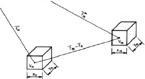
Fig. 15.25. Interrelation between the position vectors of two cubical elements inside
the body; position vectors are with respect to the assumed origin
Therefore, (15.228) b ecomes
E
m
=
E
m
i
+
→
Γ
mn
(r
m
,r
0
).
E
n
. (15.230)
Equation (15.230) can be written as
E
m
=
→
K
mn
E
n
. (15.231)
Here
→
K
mn
=
→
Γ
mn
−
→
δ
mn
(15.232)
where,
→
δ
mn
=
⎡
⎣
000
000
000
⎤
⎦
for m =n=
→
0 . (15.233)
It is t ermed as the null dyadic and
→
δ
mn
=
⎡
⎣
100
010
001
⎤
⎦
for m =n. (15.234)
It is t ermed as the identity dyadic or idem factor.
In (15.231), there are N possible values of the superscript m and there are
three components in each vector. So (15.231) represents 3N equations in 3N
unknowns
E
n
. Matrix elements are composed of the elements of the dyadic
Green’s function.
E
m
i
are calculated for each particular source geometry.
E
i
is calculated in the absence of any inhomogeneity. In the matrix form we can
write (15.231) as
[E] = [K]
−1
[E
i
] (15.235)
534 15 Numerical Methods in Potential Theory
where [K]
−1
is a 3N × 3N matrix containing the information ab out the sub-
surface geometry and the conductivity distribution. [E
i
]isa3N× 1column
vector containing information about the source and its effect on the host in
the absence of the target body. Actual value of the electric field in the inho-
mogeneity is
Eisalso3N× 1 column vector. These values of
Ecanthen
be used to calculate
E
s
(r)anywhereinthehostrockandintheair.Elab-
orate treatments on computations of dyadic Green’s tensors are available in
Tai (1971), Weidelt (1975), Raiche (1975), Meyer (1976), Beasely and Ward
(1986), Wannamaker (1984).

16
Analytical Continuation of Potential Field
In this chapter the techniques for analytical continuation of potential field are
discussed. The topics covered, related to upward and downward continuation
of po tential fields, are (i) harmonic analysis (ii) Taylor’s series expansion and
finite difference scheme (iii)Green’s theorem, Green’s function and integral
equation (iv) Peter’s areal average (v) Lagrange interpolation formula and
integral equation (vi) Green’s theorem in electromagnetic fields.
16.1 Introducti on
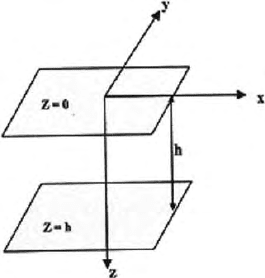
Analytical continuation of potential field is a process of finding a potential
field on any plane from the measured values of that field on any other plane
(Fig. 16.1). If a field is measured on the ground surface within a certain area,
mathematical technique of analytical continuation allows one to find out the
field on any other plane above or below the level of the plane where the
measurements were done. Continuation of the field above the level of mea-
surement is known as upward continuation. Continuation below the level of
measurement is known as downward continuation. T hese basic properties of
mathematical physics were used by the geophysicists for interpretation of field
data by upward or downward continuation. Upward continuation allows the
data to be smooth and as such there is no problem of instability in mathe-
matical continuation.
Downward continuation, on the other hand, sharpens the geophysical
anomalies in potential field and may invite instability at different levels of
continuation. Upward and downward continuation of potential fields started
in geophysics for interpretation of gravity and magnetic field data. Later appli-
cation of analytical continuation found its place in interpretation of self poten-
tial, telluric current and electromagnetic data. Aeromagnetic or aerogravity
data can be compared with upward continued gravity and magnetic potentials
recorded at a particular area. Even for downward continuation, a few units
of upward continuation is necessary. Analytical continuation of potential field
536 16 Analytical Continuation of Potential Field
Fig. 16.1. Shows two horizontal planes at a difference of height ‘h’; potentials
measured in one plane can be continued to the other plane
also comes under the broad umbrella of inversion of potential field data dis-
cussed in the next chapter.
The idea of analytical continuation of potential field in geophysics started
coming from the third decade of the last century. Authors developed this
subject are Evjen (1936), Tsuboi and Fuchida (1937), Tsuboi (1938), Hughes
(1942), Bullard and Cooper (1948), Peters (1949), Henderson and Zeitz (1949),
Trejo (1954), Roy (1960, 1962, 1963, 1966a, 1966b, 1967, 1968, 1969), (1961)
and Huestis and Parker (1979).
Different mathematical to ols used for analytical continuation are Taylor’s
series expansion, and finite difference approximation solution of Laplace equa-
tion, harmonic analysis, Green’s theorem, Fourier sine transform, relaxation,
Lagrange interp olation, integral equation and spatial averaging. The subject
originally came forward for handling gravity and magnetic data. Roy(papers
cited above) have shown that the same technique can be extended in the
fields of telluric current, self potential, direct current and electromagnetic
field of geophysical interest. Huestis and Parker (1979) have proposed the use
of Bachus-Gilbert inversion approach (1968, 1970) for analytical continuation
of p otential field. Analytical continuation of gravity and magnetic data is used
widely by geophysicists in oil and mineral industries.
In this chapter a few approaches of analytical continuation are presented
the way the different authors have proposed.
16.2 Downward Continuation by Harmonic Analysis
of Gravity Field
Tsuboi and Fuchida (1937) first suggested the harmonic analysis approach for
downward continuation of the gravity fi eld. The general solution of Laplace
equation in Cartisian coordinate is given by
16.3 Ta ylor’s Series Expansion and Finite Difference Approach 537
φ (x, y, z) =
∞
m=0
∞
n=0
A
mn
cos mx cos ny
sin mx sin my
e
√
m
2
+n
2
z (16.1)
and
∂φ
∂z
z=0
=g(x, y) . (16.2)
Here φ is the gravitational potential and g is the vertical component of the
gravity field.
From (16.1) we get
∂φ
∂z
z=0
=
∞
m=0
∞
n=0
A
mn
m
2
+n
2
.
cos mx cos ny
sin mx sin ny
(16.3)
=
∞
m=0
∞
n=0
B
mn
cos mx cos ny
sin mx sin ny
(16.4)
where
B
mn
=A
mn
m
2
+n
2
.
And
∂φ
∂z
z=d
=
∞
m=0
∞
n=0
C
mn
cos mx cos ny
sin mx sin ny
where
C
mn
=B
mn
e
√
m
2
+n
2
.d
. (16.5)
Equation (16.5) gives the downward continued gravity field.
16.3 Taylor’s Series Expansion and Finite Difference
Approach for Downward Continuation
16.3.1 Approach A
Bullard and Coopper’s approach
Bullard and Cooper (1948) suggested the finite difference approach and used
Taylor’s series expansion to obtain downward continued gravity values in a
two dimensional square grid of separation ‘a’ in a xz plane (Fig. 16.2). One
can write
g
1
=g
0
+a
∂g
∂x
+
1
2!
a
2
∂
2
g
∂x
2
+ (16.6)
g
2
=g
0
− a
∂g
∂x
+
1
2!
a
2
∂
2
g
∂x
2
− (16.7)
g
3
=g
0
+a
∂g
∂z
+
1
2!
a
2
∂
2
g
∂z
2
+ (16.8)
g
4
=g
0
− a
∂g
∂z
+
1
2!
a
2
∂
2
g
∂z
2
+ (16.9)

538 16 Analytical Continuation of Potential Field
Fig. 16.2. Finite difference cell
where g
1
,g
2
,g
3
,g
4
and g
0
are the gravity values at the p oints 1,2,3,4 and 0.
Adding equations (16.6) , (16.7) and (16.8) ,(16.9). we get
g
1
+g
2
+g
3
+g
4
≡4g (0) +
a
2
2!
∂
2
g
∂x
2
+
∂
2
g
∂z
2
+
a
4
4!
∂
4
g
∂x
4
+
∂
4
g
∂z
4
. (16.10)
For two dimensional bodies, the gravity field in a source free region satisfy
Laplace’s equation.
Hence
4g (0) = g
1
+g
2
+g
3
+g
4
(16.11)
16.3.2 Approach B
For downward continuation of two dimensional fields, we can write
g(+h)=g(0)+h
∂g
∂g
z=0
+
h
2
2!
∂
2
g
∂z
2
z=0
+
=
∞
n=0
(h)
n
n!
∂
n
g
∂z
n
z=0
. (16.12)
The general solution of the Lapla ce equation in cylindrical po l ar coordinate
is
g(r, θ, z) =
∞
n=0
k
k=1
e
µ
k
z
(A
km
cos nθ +B
km
sin nθ)J
n
(µ
k
r) (16.13)
where J
n
(µ
k
r) is the Bessel’s function of n order and first kind.
A
km
and B
km
are the kernels to be determined from the boundary condi-
tion.
For azimuthal independence of the potential field, (16.13) reduces to