Roy K.K. Potential theory in applied geophysics
Подождите немного. Документ загружается.


15.8 Galerkin’s Approach Isoparametric Elements Magnetotellurics 519
equation is
∂
∂y
1
ˆz
∂E
xs
∂y
+
∂
∂z
1
∂z
∂E
xs
∂z
− ˆyE
xs
=∆ˆyE
xp
. (15.171)
Similarly, Maxwell’s equations for the secondary components of the TM mode,
E
x
= H
y
= H
z
= ∂/∂x = 0. Here the guiding equations are
∂H
xs
∂z
=ˆyE
ys
+∆ˆyE
yp
(15.172)
∂H
xs
∂y
=ˆyE
zs
+∆ˆyE
zp
(15.173)
and
∂E
zs
∂y
−
∂E
ys
∂z
= −ˆzH
xs
. (15.174)
Substituting (15.172) and (15.173) into (15.174) and rearranging, the TM
mode Helmholtz equation one gets
∂
∂y
1
ˆy
∂H
xs
∂y
+
∂
∂z
1
ˆy
∂H
xs
∂z
− ˆzH
xs
=∆
∆k
2
ˆy
H
xp
+
∂
∂z
∆ˆy
ˆy
E
yp
(15.175)
where ∆k
2
= −∆
⌢
y
⌢
z
and E
zp
is zero in the magnetotellurics.
The (15.171) and (15.175) can be written in more general form as
∂
∂y
1
q
∂
ˆ
f
e
∂y
+
∂
∂z
∂
ˆ
f
e
∂z
+ p
⌢
f
e
− s = 0 (15.176)
where, q =ˆz, p = −ˆy,s =∆
⌢
y
E
xp
for TE-mode.
q =
⌢
y
,p= −
⌢
z
,s=
∆k
2
ˆy
H
xp
−
∂
∂z
∆ˆy
ˆy
E
yp
for TM-mode.
The(15.176) can be written as
∂
∂y
(F 1) +
∂
∂z
(F 2) + p
ˆ
f
e
− s = 0 (15.177)
where,
F1 =
1
q
∂
⌢
f
e
∂y
(15.178)
F2 =
1
q
∂
⌢
f
e
∂z
.
The element equations for finite element solution,
L
⌢
f = s (15.179)

520 15 Numerical Methods in Potential Theory
where L is the Helmholtz operator,
ˆ
f is the unknown secondary electric or
magnetic field parallel or perpendicular to the strike depending upon TE or
TM mode formulation and s is the source function. We assume that ‘
ˆ
f ’isa
piecewise lin ear functions over quadrilateral sub region ‘e’ o f the domain and
we can write
ˆ
f =
m
e=1
ˆ
f
e
(15.180)
where, m is total number of quadrilateral sub domains and,
ˆ
f
e
= α
1
+ α
2
x + α
3
y + α
4
xy + α
5
x
2
+ α
6
y
2
+ α
7
x
2
y + α
8
xy
2
. (15.181)
For node ‘ i’
ˆ
f
e
= α
1
+ α
2
x
i
+ α
3
y
i
+ α
4
x
i
y
i
+ α
5
x
i
2
+ α
6
y
i
2
+ α
7
x
i
2
y
i
+ α
8
x
i
y
i
2
. (15.182)
Having defined the form of the approximation over these domains, the error
approximation (ε) can be obtained after substituting (15.182) into (15.179)
i.e.,
L
ˆ
f − s ≡ ε. (15.183)
As discussed in Sect. 15.7, by proper choice of the weights, the error can be
minimised to zero. These weights are Galerkin’s weights. One gets
e
W
e
L
ˆ
f − s
dydz =0. (15.184)
Mathematically, this states that the error of approximation be orthogonal to
the weight functions ‘W
e
’ over each sub domain ‘e’ i.e.,
Ω
e
W
∂
∂y
(F
1
)+
∂
∂z
(F
2
)+p
ˆ
f − s
dydz =0. (15.185)
Integrating first two terms in (15.185) by parts, we get
∂
∂y
(WF
1
)=
∂W
∂y
F
1
+ W
∂F
1
∂y
(15.186)
∂
∂z
(WF
2
)=
∂W
∂z
F
2
+ W
∂F
2
∂z
. (15.187)
Equation (15.186 and 15.187) can b e written as
−W
∂F
1
∂y
=
∂W
∂y
F
1
−
∂
∂y
(WF
1
)
−W
∂F
2
∂z
=
∂W
∂z
F
2
−
∂
∂z
(WF
2
) . (15.188)
From Stokes theorem,

15.8 Galerkin’s Approach Isoparametric Elements Magnetotellurics 521
Ω
e
∂
∂y
(WF
1
) dydz =
r
e
WF
1
n
y
ds
Ω
e
∂
∂z
(WF
2
) dydz =
r
e
WF
2
n
z
ds (15.189)
where, n
y
and n
z
are the components (i.e., direction cosines) of the unit
normal vector
ˆn = n
y
i + n
z
j (15.190)
=cos(α) i +sin(α)j
on the boundary Γ
e
, and ds is the arc length of an infinitesimal line element
along the boundary. Using (15.188) and (15.189) in (15.185)
Ω
e
∂W
∂y
(F
1
)+
∂W
∂z
(F
2
)+Wp
ˆ
f − Ws
dydz (15.191)
−
Γ
e
W [n
y
(F
1
)+n
z
(F
2
)]ds =0.
Equation (15.191) can be written as
Ω
e
)
∂W
∂y
1
q
∂
ˆ
f
e
∂y
+
∂W
∂z
1
q
∂
ˆ
f
e
∂z
+ Wp
ˆ
f
e
− Ws
*
dydz (15.192)
−
Γ
e
W
)
n
y
1
q
∂
ˆ
f
e
∂y
+ n
z
1
q
∂
ˆ
f
e
∂z
*
ds =0
which is equal to
Ω
E
⎛
⎝
−
1
q
(
∂
ˆ
f
e
∂y
∂W
∂y
+
∂
⌢
f
e
∂z
∂W
∂z
)+W
p
⌢
f
e
− s
⎞
⎠
dydz
+
Γ
e
1
q
∂
ˆ
f
e
∂η
Wds ≡ 0.
(15.193)
But, in Garlerkin’s technique, the weights are equivalent to the approximate
(or shape) functions.
The (15.193) further can be written as
Ω
e
⎛
⎝
−
1
q
(
∂
ˆ
f
e
∂y
∂N
e
n
∂y
+
∂
⌢
f
e
∂z
∂N
e
n
∂z
)+N
e
n
p
⌢
f
e
− s
⎞
⎠
dydz
+
Γ
e
1
q
∂
ˆ
f
e
∂η
N
e
n
ds ≡ 0
(15.194)

522 15 Numerical Methods in Potential Theory
where,
∂
⌢
f
e
∂η
is the normal derivative of the basis function at the element bound-
ary, which is equivalent to
∂
⌢
f
e
∂η
=
∂
⌢
f
e
∂y
n
y
+
∂
⌢
f
e
∂z
n
z
(15.195)
where n
y
and n
z
are the y and z component of the unit vector normal to the
boundary. ds is the differential arc length along the boundary Ω
e
of the quadri-
lateral element. Since internal element boundaries would be traversed twice
in opposite directions during integration, the surface integral term of (15.193)
is henceforth dropped from consideration which for the external boundaries
the terms are either zero for Neumann bound ary conditions or need not be
evaluated for Dirichlet boundary conditions.
The (15.194) can be written as
(Q
e
+ P
e
)
ˆ
f
e
= S
e
(15.196)
where
Q
e
ij
= −
e
1
q
∂N
e
i
∂y
∂N
e
j
∂y
+
∂N
e
j
∂z
∂N
e
j
∂z
dydz (15.197)
P
e
ij
=
e
pN
e
i
N
e
j
dydz (15.198)
S
e
i
=
e
sN
e
i
dydz. (15.199)
15.8.3 Shape Functions Using Natural Coordinates (ξ, η )
Isoparametric formulation makes it possible to generate elements that are non-
rectangular (or) non-quradrilateral and have curved boundaries. These shapes
have obvious usage in grading a mesh from coarse to fine in modelling arbi-
trary shapes, and curved bo u n daries. In formulating isoparametric elements,
natural coordinate system (ξ,η) may be used. Secondary fields are expressed
in terms of natural coordinates, but must be differentiated with respect to
global coordinate y and z.
A non-rectangular region cannot be represented by using rectangular ele-
ment; however, it can b e represented by quadrilateral elements. Since, the
interp olation function are easily derivable for a rectangular element, and it
is easy to evaluate integrals over rectangular geometries, we transform the
finite element integrals defined over quadrilaterals to rectangles. Therefore,
numerical integration schemes, such as Gauss–Legendre scheme, require that
15.8 Galerkin’s Approach Isoparametric Elements Magnetotellurics 523
the integral b e evaluated on a specific domain or with respect to specific
coordinate system. The transformation of the geometry and the variable coef-
ficients of the differential equation from the problem coordinates (x, y) to the
natural co ordinates (ξ,η) results in algebraically complex expression and this
precludes analytical (i.e., exact) evaluation of the integrals. Thus, the trans-
formation of a given integral expression is defined over the element Ω
e
,toone
of the domain
⌢
Ω
and must be such as to facilitate numerical integration. Each
element of the finite element mesh is transformed to
⌢
Ω
, only for the purposes
of numerically evaluating the integrals. The element Ω
e
, is called a master
element.
The transformation between Ω
e
and
⌢
Ω
i.e., between (x, y) and (ξ,η)is
accomplished by a co ordinate transformation of the form.
y =
8
i=1
N
i
y
i
(15.200)
z =
8
i=1
N
i
z
i
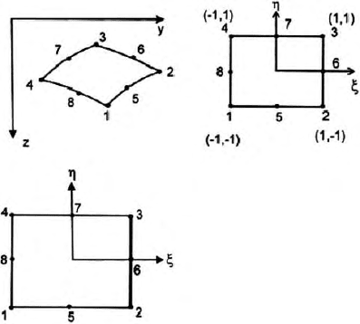
for eight noded isoparametric element, axes ξ and η pass through mid points
of opposite sides as shown in (Fig. 15.22). Axes ξ and η need be orthogonal,
and neither need be parallel to the y-axis nor the z-axis. Side of the element
are at ξ = ±1andη = ±1. The interpolation (or shape) functions following
Sect. 15.8.1 can be worked out to be
Fig. 15.22. Advanced level eight nodded isoparametric element

524 15 Numerical Methods in Potential Theory
For no de 1:
1
4
(1 −ξ)(1− η)(−ξ −η −1)
For no de 2:
1
4
(1 + ξ)(1− η)(ξ − η − 1)
For no de 3:
1
4
(1 + ξ)(1+η)(ξ + η − 1)
For no de 4:
1
4
(1 −ξ)(1+η)(−ξ + η − 1)
For no de 5:
1
2
1 −ξ
2
(1 −η)
For no de 6:
1
2
(1 + ξ)
1 −η
2
For no de 7:
1
2
1 −ξ
2
(1 + η)
For no de 8:
1
2
(1 −ξ)
1 −η
2
15.8.4 Coordinate Transformation
The transformation of a quadrilateral element of a finite element mesh to
the master element
⌢
Ω
is solely for the purpose of numerically evaluating the
integrals (15.197), (15.198), (15.199). The resulting algebraic equations of the
finite element formulations are always among the nodal values of the physical
domain. Different element of the finite element mesh can be generated from
the same master element by assigning the global co ordinates of the elements.
With the help of an appropriate master element, any arbitrary element of
a mesh can be generated. However, the transformation of a master element
should b e such that there are no spurious gaps between elements and no
element overlaps.
When a typical element of the finite element mesh is transformed to its
master element for the purpose of numerically evaluating integrals, the inte-
grand must also be expressed in terms of coordinates (ξ, η) of the master ele-
ment. In the (15.194), the integrand i.e., the expression in the square brackets
under the integral) and their derivatives are functions of the global coordi-
nates y and z.. We must rewrite it in terms of (ξ)and(η) using transformation
(15.160 to 15.165).
Therefore, we must relate
∂N
e
i
∂y
and
∂N
e
i
∂z
to
∂N
e
i
∂ξ
and
∂N
e
i
∂η
.
The function N
e
i
can be expressed in terms of the lo cal coordinates ξ and
η by means of (15.194). Hence, by chain rule of partial differentiation, we
have
∂N
e
i
∂ξ
=
∂N
e
i
∂y
∂y
∂ξ
+
∂N
e
i
∂z
∂z
∂ξ
(15.201)
∂N
e
i
∂η
=
∂N
e
i
∂y
∂y
∂η
+
∂N
e
i
∂z
∂z
∂η
.
In matrix notation
⎛
⎝
∂N
e
i
∂ξ
∂N
e
i
∂η
⎞
⎠
=
∂y
∂ξ
∂z
∂ξ
∂y
∂η
∂z
∂η
⎛
⎝
∂N
e
i
∂y
∂N
e
i
∂z
⎞
⎠
(15.202)

15.8 Galerkin’s Approach Isoparametric Elements Magnetotellurics 525
which gives the relation between the derivatives N
e
i
with respect to the global
and local coordinates. The (15.202) can be written as
⎛
⎝
∂N
e
i
∂ξ
∂N
e
i
∂η
⎞
⎠
=[J]
⎛
⎝
∂N
e
i
∂y
∂N
e
i
∂z
⎞
⎠
(15.203)
where, [J] is known as Jacobian matrix which is equal to
[J]=
∂y
∂ξ
∂z
∂ξ
∂y
∂η
∂z
∂η
. (15.204)
To find the cartesian derivatives of N
e
i
,weget
⎛
⎝
∂N
e
i
∂y
∂N
e
i
∂z
⎞
⎠
=[J]
−1
⎛
⎝
∂N
e
i
∂ξ
∂N
e
i
∂η
⎞
⎠
(15.205)
=
1
|J|
∂z
∂η
−
∂z
∂ξ
−
∂y
∂η
∂y
∂ξ
⎛
⎝
∂N
e
i
∂ξ
∂N
e
i
∂η
⎞
⎠
where,
|J| =
∂y
∂ξ
∂z
∂η
−
∂y
∂η
∂z
∂ξ
. (15.206)
This requires that the Jacobian matrix [J] b e non-singular.
The (15.206) can be written as
∂N
e
i
∂y
=
∂N
e
i
∂ξ
∂ξ
∂y
+
∂N
e
i
∂η
∂η
∂y
(15.207)
∂N
e
i
∂z
=
∂N
e
i
∂ξ
∂ξ
∂z
+
∂N
e
i
∂η
∂η
∂z
.
From (15.202), the (15.204) will b e
[J]=
⎛
⎜
⎜
⎝
8
4
i=1
∂N
i
∂ξ
x
i
8
4
i=1
∂N
i
∂ξ
x
i
8
4
i=1
∂N
i
∂ξ
x
i
8
4
i=1
∂N
i
∂ξ
x
i
⎞
⎟
⎟
⎠
. (15.208)
Equation (15.206) can be restructured as
[J]=
⎛
⎝
∂N
1
∂ξ
∂N
2
∂ξ
∂N
3
∂ξ
∂N
4
∂ξ
∂N
5
∂ξ
∂N
6
∂ξ
∂N
7
∂ξ
∂N
81
∂ξ
∂N
1
∂η
∂N
2
∂η
∂N
3
∂η
∂N
4
∂η
∂N
5
∂η
∂N
6
∂η
∂N
7
∂η
∂N
81
∂η
⎞
⎠
⎛
⎜
⎜
⎜
⎜
⎜
⎜
⎜
⎜
⎜
⎜
⎝
x
1
y
1
x
2
y
2
x
3
y
3
x
4
y
4
x
5
y
5
x
6
y
6
x
7
y
7
x
8
y
8
⎞
⎟
⎟
⎟
⎟
⎟
⎟
⎟
⎟
⎟
⎟
⎠
. (15.209)

526 15 Numerical Methods in Potential Theory
The element area d A = dydz in the element Ω
e
is transformed to
dA = dydz = |J|dξdη (15.210)
in the master element
⌢
Ω
.
Equation (15.197), (15.198) and (15.199) can be written as
Q
e
ij
= −
1
−1
1
q
∂N
e
i
∂ξ
∂N
e
j
∂ξ
|J|dξdη −
1
−1
1
q
∂N
e
i
∂ξ
∂N
e
j
∂ξ
|J|dξdη (15.211)
P
e
ij
= pN
e
i
N
e
j
|J|dξdη (15.212)
and
S
e
ij
= sN
e
i
|J|dξdη (15.213)
the (15.209) can be written as
Q
e
ij
= Q1
e
ij
+ Q2
e
ij
(15.214)
where
Q1
e
ij
=
⎛
⎜
⎜
⎜
⎜
⎜
⎜
⎜
⎜
⎜
⎜
⎜
⎜
⎜
⎜
⎜
⎜
⎜
⎜
⎜
⎜
⎜
⎜
⎜
⎜
⎜
⎜
⎜
⎜
⎜
⎝
∂N
1
∂ξ
∂N
1
∂ξ
∂N
1
∂ξ
∂N
2
∂ξ
∂N
1
∂ξ
∂N
3
∂ξ
∂N
1
∂ξ
∂N
4
∂ξ
∂N
1
∂ξ
∂N
5
∂ξ
∂N
1
∂ξ
∂N
6
∂ξ
∂N
1
∂ξ
∂N
7
∂ξ
∂N
1
∂ξ
∂N
8
∂ξ
∂N
2
∂ξ
∂N
1
∂ξ
∂N
2
∂ξ
∂N
2
∂ξ
∂N
2
∂ξ
∂N
3
∂ξ
∂N
2
∂ξ
∂N
4
∂ξ
∂N
2
∂ξ
∂N
5
∂ξ
∂N
2
∂ξ
∂N
6
∂ξ
∂N
2
∂ξ
∂N
7
∂ξ
∂N
2
∂ξ
∂N
8
∂ξ
∂N
3
∂ξ
∂N
1
∂ξ
∂N
3
∂ξ
∂N
2
∂ξ
∂N
3
∂ξ
∂N
3
∂ξ
∂N
3
∂ξ
∂N
4
∂ξ
∂N
3
∂ξ
∂N
5
∂ξ
∂N
3
∂ξ
∂N
6
∂ξ
∂N
3
∂ξ
∂N
7
∂ξ
∂N
3
∂ξ
∂N
8
∂ξ
∂N
4
∂ξ
∂N
1
∂ξ
∂N
4
∂ξ
∂N
2
∂ξ
∂N
4
∂ξ
∂N
1
∂ξ
∂N
4
∂ξ
∂N
1
∂ξ
∂N
4
∂ξ
∂N
1
∂ξ
∂N
4
∂ξ
∂N
1
∂ξ
∂N
1
∂ξ
∂N
1
∂ξ
∂N
1
∂ξ
∂N
1
∂ξ
∂N
5
∂ξ
∂N
1
∂ξ
∂N
5
∂ξ
∂N
2
∂ξ
∂N
5
∂ξ
∂N
1
∂ξ
∂N
5
∂ξ
∂N
1
∂ξ
∂N
5
∂ξ
∂N
1
∂ξ
∂N
5
∂ξ
∂N
1
∂ξ
∂N
1
∂ξ
∂N
1
∂ξ
∂N
1
∂ξ
∂N
1
∂ξ
∂N
6
∂ξ
∂N
1
∂ξ
∂N
6
∂ξ
∂N
2
∂ξ
∂N
6
∂ξ
∂N
1
∂ξ
∂N
6
∂ξ
∂N
1
∂ξ
∂N
6
∂ξ
∂N
1
∂ξ
∂N
6
∂ξ
∂N
1
∂ξ
∂N
1
∂ξ
∂N
1
∂ξ
∂N
1
∂ξ
∂N
1
∂ξ
∂N
7
∂ξ
∂N
1
∂ξ
∂N
7
∂ξ
∂N
2
∂ξ
∂N
7
∂ξ
∂N
1
∂ξ
∂N
7
∂ξ
∂N
1
∂ξ
∂N
7
∂ξ
∂N
1
∂ξ
∂N
7
∂ξ
∂N
1
∂ξ
∂N
1
∂ξ
∂N
1
∂ξ
∂N
1
∂ξ
∂N
1
∂ξ
∂N
8
∂ξ
∂N
1
∂ξ
∂N
8
∂ξ
∂N
2
∂ξ
∂N
8
∂ξ
∂N
1
∂ξ
∂N
8
∂ξ
∂N
1
∂ξ
∂N
8
∂ξ
∂N
1
∂ξ
∂N
8
∂ξ
∂N
1
∂ξ
∂N
1
∂ξ
∂N
1
∂ξ
∂N
1
∂ξ
∂N
1
∂ξ
⎞
⎟
⎟
⎟
⎟
⎟
⎟
⎟
⎟
⎟
⎟
⎟
⎟
⎟
⎟
⎟
⎟
⎟
⎟
⎟
⎟
⎟
⎟
⎟
⎟
⎟
⎟
⎟
⎟
⎟
⎠
(15.215)

15.8 Galerkin’s Approach Isoparametric Elements Magnetotellurics 527
and Q2
e
ij
=
⎛
⎜
⎜
⎜
⎜
⎜
⎜
⎜
⎜
⎜
⎜
⎜
⎜
⎜
⎜
⎜
⎜
⎜
⎜
⎜
⎜
⎜
⎜
⎜
⎜
⎜
⎜
⎜
⎜
⎜
⎝
∂N
1
∂ξ
∂N
1
∂ξ
∂N
1
∂ξ
∂N
2
∂ξ
∂N
1
∂ξ
∂N
3
∂ξ
∂N
1
∂ξ
∂N
4
∂ξ
∂N
1
∂ξ
∂N
1
∂ξ
∂N
1
∂ξ
∂N
1
∂ξ
∂N
1
∂ξ
∂N
1
∂ξ
∂N
1
∂ξ
∂N
1
∂ξ
∂N
2
∂ξ
∂N
1
∂ξ
∂N
1
∂ξ
∂N
1
∂ξ
∂N
1
∂ξ
∂N
1
∂ξ
∂N
1
∂ξ
∂N
1
∂ξ
∂N
1
∂ξ
∂N
1
∂ξ
∂N
1
∂ξ
∂N
1
∂ξ
∂N
1
∂ξ
∂N
1
∂ξ
∂N
1
∂ξ
∂N
1
∂ξ
∂N
3
∂ξ
∂N
1
∂ξ
∂N
1
∂ξ
∂N
1
∂ξ
∂N
1
∂ξ
∂N
1
∂ξ
∂N
1
∂ξ
∂N
1
∂ξ
∂N
1
∂ξ
∂N
1
∂ξ
∂N
1
∂ξ
∂N
1
∂ξ
∂N
1
∂ξ
∂N
1
∂ξ
∂N
1
∂ξ
∂N
1
∂ξ
∂N
4
∂ξ
∂N
1
∂ξ
∂N
1
∂ξ
∂N
1
∂ξ
∂N
1
∂ξ
∂N
1
∂ξ
∂N
1
∂ξ
∂N
1
∂ξ
∂N
1
∂ξ
∂N
1
∂ξ
∂N
1
∂ξ
∂N
1
∂ξ
∂N
1
∂ξ
∂N
1
∂ξ
∂N
1
∂ξ
∂N
1
∂ξ
∂N
5
∂ξ
∂N
1
∂ξ
∂N
1
∂ξ
∂N
1
∂ξ
∂N
1
∂ξ
∂N
1
∂ξ
∂N
1
∂ξ
∂N
1
∂ξ
∂N
1
∂ξ
∂N
1
∂ξ
∂N
1
∂ξ
∂N
1
∂ξ
∂N
1
∂ξ
∂N
1
∂ξ
∂N
1
∂ξ
∂N
1
∂ξ
∂N
6
∂ξ
∂N
1
∂ξ
∂N
1
∂ξ
∂N
1
∂ξ
∂N
1
∂ξ
∂N
1
∂ξ
∂N
1
∂ξ
∂N
1
∂ξ
∂N
1
∂ξ
∂N
1
∂ξ
∂N
1
∂ξ
∂N
1
∂ξ
∂N
1
∂ξ
∂N
1
∂ξ
∂N
1
∂ξ
∂N
1
∂ξ
∂N
7
∂ξ
∂N
1
∂ξ
∂N
1
∂ξ
∂N
1
∂ξ
∂N
1
∂ξ
∂N
1
∂ξ
∂N
1
∂ξ
∂N
1
∂ξ
∂N
1
∂ξ
∂N
1
∂ξ
∂N
1
∂ξ
∂N
1
∂ξ
∂N
1
∂ξ
∂N
1
∂ξ
∂N
1
∂ξ
∂N
1
∂ξ
∂N
8
∂ξ
∂N
1
∂ξ
∂N
1
∂ξ
∂N
1
∂ξ
∂N
1
∂ξ
∂N
1
∂ξ
∂N
1
∂ξ
∂N
1
∂ξ
∂N
1
∂ξ
∂N
1
∂ξ
∂N
1
∂ξ
∂N
1
∂ξ
∂N
1
∂ξ
∂N
1
∂ξ
∂N
1
∂ξ
∂N
1
∂ξ
⎞
⎟
⎟
⎟
⎟
⎟
⎟
⎟
⎟
⎟
⎟
⎟
⎟
⎟
⎟
⎟
⎟
⎟
⎟
⎟
⎟
⎟
⎟
⎟
⎟
⎟
⎟
⎟
⎟
⎟
⎠
(15.216)
For i = 1 to 8, ∂N
i
/∂ξ is
∂N
1
∂ξ
=
(1 − η)(2ξ + η)
4
∂N
2
∂ξ
=
(1 − η)(2ξ − η)
4
(15.217)
∂N
3
∂ξ
=
(1 + η)(2ξ + η)
4
∂N
4
∂ξ
=
(1 + η)(η − 2ξ)
4
∂N
5
∂ξ
= −ξ (1 − η)
∂N
6
∂ξ
=
1 −η
2
2
∂N
7
∂ξ
= −ξ (1 + η)
∂N
8
∂ξ
= −
1 −η
2
2
.
Similarly, for i = 1 to 8, ∂N
i
/∂η is

528 15 Numerical Methods in Potential Theory
∂N
1
∂η
=
(1 − ξ)(2η + ξ)
4
∂N
2
∂η
=
(1 + ξ)(ξ −2 η)
4
(15.218)
∂N
3
∂η
=
(1 + ξ)(2η + ξ)
4
∂N
4
∂η
=
(1 − ξ)(2η − ξ)
4
∂N
5
∂η
= −
1 −ξ
2
2
∂N
6
∂η
= −η (1 + ξ)
∂N
7
∂η
= −
1 −ξ
2
2
where, q, p and s depend upon whether TE or TM modes are being consid-
ered fo r e valuation. All the elements of the matrices are to be o btained using
numerical integration using Gauss Legender Quadrature . Gauss weights for
one two and three dimensional problems are available in standard mathemat-
ical handbooks.One chooses 3,5,7,9 point Gauss Quadrature depending upon
the accuracy needed. The steps includ e: generation of element matrices Q
e
,P
e
and S
e
as defined in (15.197), (15.198) and (15.199) respectively. These ele-
ment matrices are assembled to form the global matrix, before imp osition of
boundary conditions. The nodal field variables are obtained by solving the
finite element equations.
15.9 Integral Equation Method
15.9.1 Introduction
An equation, where an unknown function to be determined, remains within
the integral sign, is an integral equation. The integral equations are defined
by Fredhom and Volterra. Fredhom and Volterra’s integral equations of the
first, second and third kind are given by the (2.46, 2.47, 2.48, 2.49, 2.50, 2.51)
Often the Kernel functions of these integral equations are Green’s function. If
the limits of these integral are finite, the integrals are of Fredhom type. For
an infinite or undefined limits of the integral, the integral equations are of
Vo lterra’s type. Geophysical Boundary value problems solved using integral
equations generally appear in the form of Fredhom’s integral equation of the
second kind.
f(r) − λ
v
G(r, r
0
)f(r
0
)dv
0
= g(r) (15.219)
where G(r, r
0
) is the Green’s function with observation points and source
points are respectively at r and r
0
; g(r) is the known function and f(r) is the