Roy K.K. Potential theory in applied geophysics

Подождите немного. Документ загружается.

16.5 Analytical Continuation using Integral Equation 549

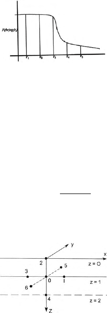
Fig. 16.8. Variation of f(hr) with radial distance

Table 16.1, the co eﬃcients for continuation downward can b e obtained for

h = 1 and h = 2. These coeﬃcients are given in Table 16.2 and are used along

with the values given (Fig. 16.8).

Trejo (1954) suggested that one can get better results for downward con-

tinuation if Peters upward continuation program and three dimensional ﬁnite

diﬀerence program is used together for downward continuation. His working

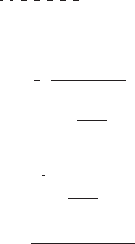
relation is (Fig. 16.9)

g(0, 0, h) =6g(0, 0, 0) − g(h, 0, 0) − g(−h, 0, 0)

− g(0, h, 0) − g(0, −h, 0) − g(0, 0 − h). (16.51)

This relation gives the value of g at a depth h in terms of the measured values

of g at a height −h, and at the ﬁve points on the surface z = 0.

g(0, 0, h) = −

∞



¯g(r)hrdr

)

3/2

(16.52)

is valid only for negative non-zero values of h. At h = 0, the expression on

the right side of the expression is not well deﬁned. Baranov (1953) argued

that if this expression could be made to behave properly at h = 0, s uch

Fig. 16.9. Finite diﬀerence grid points at three diﬀerent levels

550 16 Analytical Continuation of Potential Field

that it yields th e observed g (0,0) at that point, then one could extrapo-

late g (0, h) backwards, so to say to positive value of h and achieve down-

ward continuation. Baranov was able to do this by breaking up the range

of integration in to 10 intervals expressing ¯g (r) in suitable polynomials

and then determining the constants of the polynomial in terms of ¯g(r) at

r=0, 1,

√

10,

√

17,

√

25,

√

40,

√

68, 10.

16.6 Upward and Downward Continuation using Integral

Equation and Lagrange Interpolation Formula

Henderson and Zeitz (1949) independently suggested the approach for upwa rd

continuation which is also based on the integral which connects the gravity o r

magnetic ﬁelds at diﬀerent levels, i.e.,

g(α, β, −h) =

2π

∞



−∞

g(x, y, 0) dxdy



(x −α)

+(y− β)



3/2

. (16.53)

This equation is valid for upward continuation. In cylindrical coordinate it is

g(α, β, −h) =

∞



¯g(r)hrdr

)

3/2

. (16.54)

Equation (16.54) can b e written as

n−1



i=1

¯g(r)f(r

, h) (r

i+1

− r

i−1

) (16.55)

g(r

)f(r

, h) (r

n+1

− r

n−1

)

where

f(r

, h) =

)

3/2

. (16.56)

Using equation (16.53), g(0, 0, −h), the upward continued values of the grav-

itational ﬁeld can be calculated using the Lagrange interpolation polynomial

g(0, 0, −h) =



m=0

(−1)

h(h+s)(h+2s).........(h + ns)

(h + ms) (n −m)!m!

g(−ms) .

(16.57)

Here S is the grid spacing and n is the highest value of m.

Henderson and Zeitz (1949) used Lagrange’s interpolation formula for

downward continuation. If the anomaly on the plane of observation and

16.7 Downward Continuation of Telluric Current Data 551

upward continuation at 5 heights each of one grid spacing apart are known,

the gravity ﬁeld at a depth ‘h’ can be determined from the formula

g(0, 0, −h) =



n=0

(−1)

h(h+a)(h+2a).........(h + na)

(h + ma) (n −m)!n!

. (16.58)

Equation (16.57) and (16.58) are same. The sign of ‘h’ will dictate whether the

continuation is upward or downward. For downward continuation the maxi-

mum value of n is taken as 5. That is 5 units of upward continuation is nec-

essary for downward continuation from g eneral solution of Laplace equation

and Taylor’s series expansion.

16.7 Downward Continuation of T elluric Current Data

Earth currents or telluric currents are continuously ﬂowing through the con-

ducting portion of the upper crust. These currents are induced on the earth by

electromagnetic waves which are propagated from the magnetosphere towards

the surface of the earth. These currents are ﬂowing through the subsurface as

if the currents are generated by two inﬁnitely long line electrodes placed at

inﬁnite distance and this electrode pair is continuously rotating to generate

elliptically or circularly polarized telluric ﬁelds.

For telluric current ﬂow it is assumed that a perfectly insulating basement

is overlain by a homogeneous conducting layer of sediments through which the

telluric current ﬂows. Since



∂φ

∂z



, the derivative of telluric potential normal

to the ground surface at z = 0, is zero everywhere, it follows that

∂

∂z

= −



∂

∂x

∂

∂y



∂φ

∂z

= 0 (16.59)

on the ground surface. Simil arly it can be shown that all the higher odd

derivatives are also zero on the ground surface. The Taylor’s series expansion

of (16.39), simpliﬁes to

φ (±h) = φ (0) +

∂

∂z



z=0

∂

∂z



z=0

+ (16.60)

where φ is the DC telluric potential. Although telluric ﬁeld is a time vary-

ing ﬁeld, the frequencies are very low in general. Therefore both static and

dynamic theories are used with equal validity to analyse earth’s natural elec-

tromagnetic ﬁeld signals. Static theory is used to study the electrotelluric

ﬁelds and potentials, dynamic theory is used in magnetotellurics although the

frequencies of the signals may be of the same order. Laplace equation is used

to study electrotellurics,

Helmholtz electromagnetic wave equation ∇

H = γ

H is used in magne-

totellurics neglecting the displacement current component in the propagation

constant γ (i.e. γ =

√

iωµσ).

552 16 Analytical Continuation of Potential Field

The continuation in this case is thus independent of the sign of h and

can be carried out very easily. One ca n directly apply the ﬁnite diﬀerence

form of Laplace’s equation to the measured data in order to obtain downward

continued potentials step by step. Speciﬁcally for two dimensional problem.

φ (0, 1) = φ (4) = φ (2) = 2φ (0) − [φ (1) + φ (3)] /2, for the ﬁrst unit of

depth of continuation and

φ(0,n)=φ(4) = 4φ(0) − φ(1) − φ(2) − φ(3) (16.61)

will be the working formula for subsequent units of depth of continuation. For

three dimensional case

φ (0, 1) ≡ φ (4) = φ (2) = 3φ (0) −[φ (1) + φ (3) + φ (5) + φ (6)] /2 (16.62)

for the ﬁrst units of the depth of continuations and

φ (0, n) ≡ φ (4) = 6φ (0) −[φ (1) + φ (2) + φ (3) + φ (4) + φ (5)] (16.63)

for the subsequent units.

After having ob t ained the downward continued potentials of a suﬃciently

large number o f levels, one can draw the equip otential contours in suitable

section. In the same vertical section one can draw the streamlines which are

orthogonal to the equipotentials. One of these stream lines correspond to the

basement surface, since the top of the basement also happens to be a ﬂ ow

surface where

∂φ

∂n

= 0. Without any other information, it is not possible to

decide which of the streamlines actually represent the basement topography.

If the depth to the top of the basement is known aprior or is determined by

magnetotelluric sounding at one point, one can ﬁnd out the entire topography

of the basement surface by choosing that ﬂow surface which passes through

the known points.

16.8 Upward and Downward Continuatio n

of Electromagnetic Field Data

Roy (1966, 1968) prescrib ed the methodology for upward continuation of elec-

tromagnetic ﬁeld starting from the Helmholtz electromagnetic wave equation

∇



ψ = γ



ψ (16.64)

where



ψ is the complex electromagnetic ﬁeld potential and γ is the propagation

constant





iωµ (σ +iωε)



. Ψ can b e expressed as



ψ =



+ i



.HereR

and I respectively represent real and imaginary comp onents. ω, µ, σ,andε,and

√

i are standard notation, in electromagnetics and are available in Chaps. (12

and 13). It can be shown that the value o f



ψ at any interior point P (x

′

)

16.8 Upward and Downward Continuation of Electromagnetic Field Data 553

(see Chap. 10) is given by those on the su rface S according to the Green’s

formula

Ψ(x

′

, y

′

, z

′

4π





∂Ψ

∂n

−γr

− Ψ

∂

∂n



−γr



ds. (16.65)

Based on two important assumptions the Helmholtz electromagnetic wave

equation reduces to Laplace equation. These assumptions are

(a) the frequencies of the electromagnetic signals with which geophysicists

work are very much on the lowe r side to achieve reasona ble skin depth

or the depth of penetration of the em signals. At those frequencies, con-

duction currents dominate over the displacement current. Therefore the

propagation constant changes to the form γ =

√

iωµσ neglecting the con-

tributions from the displacement currents.

(b) The second assumption is electrical condu ctivity of the basement is more

than two order of magnitude less than that of the sedimentary overburden.

Therefore conductivity of the basement is assumed to be zer o. Since γ =0

for σ = 0 and Helmoholtz equation reduces to Laplace equation. Therefore

the formula applicable for static or stationery cases are also applicable for

special cases in electromagnetics.

Let r =



(x − x

′

)

+(y− y

′

)

+(z− z

′

)



1/2

is the distance of P from a

surface dS at (x, y, z). Since, by the electromagnetic uniqueness theorem,

Ψ(x

′

, y

′

, z

′

) is completely determined once Ψ is deﬁned on the surface.

If is now possible to eliminate

∂Ψ

∂n

. Let us now consider Green’s second

identity





Ψ∇

φ −φ∇



dv =





∂φ

∂n

− φ

∂Ψ

∂n



ds (16.66)

where φ and Ψ are two scalar functions of position that have continuous ﬁrst

and second derivative (Chap. 10) throughout the region R and on the surface

S. Now if both φ and Ψ are harmonic then (16.66) changes to the form





∂φ

∂n

− φ

∂Ψ

∂n



ds. (16.67)

This is the reciprocity theorem, valid in the same form for two electromag-

netic ﬁelds as it is for two static and stationary ﬁelds. Multiplying (16.66) by



4π



and adding to (16.67), we get

ψ (x

′

4π





∂ψ

∂n



−γr

− φ



− ψ

∂

∂n



−γr

− φ



. (16.68)

554 16 Analytical Continuation of Potential Field

If φ is chosen so that, in a ddition to satisfying (16.68), it also assumes the

value of



−γr



on the boundary S,(16.68) reduces to

Ψ(x

′

, y

′

, z

′

4π



∂

∂n



−γ r

− φ



ds. (16.69)

Thus

∂Ψ

∂n

has been eliminated from the (16.69) at the cost of introducing

Green’s function as already mentioned. The homogeneous and isotropic vol-

ume v can now be identiﬁed with geometry as shown in (Fig. 16.6).

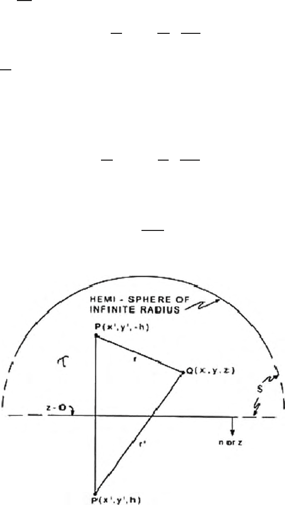
Let ‘r’ denote the radial distance of the region of air (z < 0) bounded by

a horizontal plane at z = 0 (ground surface) and an inﬁnite hemisphere above

it (Fig. 16.10). For this geometry equation (16.69) can be rewritten as

Ψ(x

′

, y

′

, z

′

= −h) = −

4π



z=0

∂

∂z



−γ r

− φ



dx dy. (16.70)

Since the integral does not vary on the inﬁnite hemisphere, the required func-

tion φ, in this case, is obviously

φ =

−γ r

′

(16.71)

Fig. 16.10. Geometry of the hemispherical space

16.8 Upward and Downward Continuation of Electromagnetic Field Data 555

where



(x −x

′

)

+(y− y)

+(z+h)



1/2

(16.72)

and

′



(x − x

′

)

+(y− y

′

)

+(z− h)



1/2

Substitution of (16.71 and 16.72) in (16.70) and diﬀerentiation yield

Ψ(x

′

, y

′

, −h) =

2π



z=0



− iγ

−γR

Ψ(x, y , 0)



dx dy (16.73)

where



(x − x

′

)

+(y− y

′

)



1/2

. (16.74)

For static and stationary ﬁelds, γ = 0 and (16.73) reduces to the well known

upward continuation integral. It is also known as the Poisson’s integral.

Since γ, the propagation constant can be written as γ = α +iβ where the

values of α and β are given in (13.13) and (13.14) We can write

exp (iγR) = exp (−βr) , (cos (αβ) + iSin (αR)) . (16.75)

The real and imaginary parts of the electromagnetic upward continuation,

integral (16.73) are therefore, given as

′

, y

′

, −h) =

2π



z=0

−βR



(x, y, 0)



β +



cos (αR)

+α sin (αR)}−Ψ

(x, y, 0)



β +



sin (αR)

−α cos (αR)]

dx dy (16.76)

′

, y

′

, −h) =

2π



z=0

−βR



β +



sin αR − α cos (αR)



+Ψ

(x, y, 0)



β +



cos αR+α sin (αR)



dx dy



dy dx. (16.77)

In air, σ = β =0,andα =w/c=

2π

, where c is the velo city of propagation

and λ is the wave length. Considering the or igin to be located on the surface

vertically below p, one has

556 16 Analytical Continuation of Potential Field

(0, 0, −h) =

2π



z=0

−βR

[Ψ

(x, y, 0)



cos



2πR



2π

sin



2πR



(16.78)

−Ψ

(x, y, 0) =



sin



2πR



−

2π

cos



2πR



dx dy (16.79)

(0, 0, −h)=

2π



z=0

[Ψ

(x, y, 0)



sin



2πR



−

2π

cos



2πR



(16.80)

+Ψ

(x, y, 0) =

2π



z=0

[Ψ

(x, y, 0)



cos



2πR



2π

sin



2πR



⎤

⎦

dx dy

where R = (x

)

1/2

. For static ﬁeld where γ =0,λ = ∞,Ψ

(x,y,0),

(16.79) and (16.80) reduces to the static upward continuation integral.

16.9 Downward Continuation o f Electromagnetic Field

Roy’s (1969) formulation for downward continuation is presented here. If the

xy plane at z = 0 (z positive downward) represents the air earth boundary,

it is known that both tangential components o f the magnetic ﬁeld H

and

and the normal comp onent H

will be continuous across the bounda ry

provided µ

air

= µ

earth

= µ

vacuum

where µ is the magnetic permeability of

the medium. Horizontal derivatives of all orders of H

and H

are also

continuous across the boundary. Since these derivatives are determined solely

from the ﬁeld values of z = 0. If we combine these back ground with the

relation.

div



∂H

∂x

∂H

∂y

∂H

∂z

= 0 (16.81)

on either side of z = 0 (air earth boundary), it follows that

∂H

∂z

is also con-

tinuous across this plane, Higher order vertical derivatives are discontinuous

across the air earth boundary since they satisfy Helmholtz electromagnetic

wave equations

∇



= γ



(in air) (16.82)

∇



= γ



(in earth) (16.83)

where γ

= µ

εω

and γ

=iωµ

(σ +iωε), µ

is the magnetic permea bility of

the vacuum. The subscripts ‘a’ and ‘e’ relate to quantities in air and in earth

immediately on two sides of the interface at z = 0. Since

16.9 Downward Continuation of Electromagnetic Field 557

∂



∂x

∂



∂x

(16.84)

∂



∂y

∂



∂y

(16.85)

and

it follows from (16.82) and (16.83) that

∂

∂z



− γ



∂

∂z

at z = 0. (16.86)

Replacing H

in (16.84) and (16.85) in turn by

∂H

∂z

∂

∂z

andsoonand

using the fact that

∂

∂x

∂z

∂

∂x

∂z

∂

∂y

∂z

∂

∂y

∂z

and

∂H

∂z

∂H

∂z

(16.87)

for higher order derivatives , one can show that

∂

∂z



− γ



∂H

∂z

∂

∂z

at z = 0

∂

∂z



− γ





− γ



∂

∂z

∂

∂z

at z = 0

∂

∂x



− γ



∂H

∂z



− γ



∂

∂z

∂

∂z

at z = 0 (16.88)

andsoon.

In general, for n = 1, 2, 3

∂

∂z





− γ



∂

∂z

at z = 0 (16.89)

and so on. On the ground, for n = 1, 2, 3

∂

2n+1

∂z

2n+1





− γ



∂

∂z

∂H

∂z

, at z = 0 (16.90)

where the superscript n indicates that the operation within the brackets has

to be carried out n terms successively.

∂H

∂z

is continuous across the boundary

∂H

∂z

and

∂H

∂z

are not b ecause

∂H

∂y

−

∂H

∂z

=iωε

(in air) (16.91)

558 16 Analytical Continuation of Potential Field

and

∂H

∂y

−

∂H

∂z

=(σ +iωε

(in earth), (16.92)

since E

and

∂H

∂y

∂H

∂y

at z = 0.

We have

∂H

∂z

∂H

∂y

σ +iωε

ωε



∂H

∂y

−

∂H

∂z

at z = 0. (16.93)

Replacing H

for H

in (16.92) and (16.93) yields

∂

∂z



− γ



∂

∂z

at z = 0. (16.94)

It can also be shown that

∂

∂z



− γ

∂

∂z



∂H

∂y

σ +iωε

ωε



∂H

∂y

−

∂H

∂z



(16.95)

at z = 0

where the operations indicated in the ﬁrst parentheses are to be carried out

over the quantity in the squared brackets. In general again for n = 1, 2, 3,.....

∂

∂z



− γ

∂

∂z



at z = 0 (16.96)

∂

∂z

2n+1



− γ

∂

∂z





∂H

∂y

σ +iωε

ωε



∂H

∂y

−

∂H

∂z



at z = 0. (16.97)

With the superscript n having the same meaning as in expression (16.84)

(16.85) and (16.86). Similar expressions can be derived for the vertical deriva-

tives of H

. In case it is the electric ﬁeld components that are observed, one

has (Stratton, 1941, p 483).

, E





(16.98)

at z = 0. From the divergence relation

∂E

∂x

∂E

∂y

∂E

∂z

= 0 (16.99)

which holds on both the sides of z = 0, it is obvious that

∂E

∂z

, like

∂H

∂z

continuous across the boundary. However as in the magnetic case,

∂E

∂z

and

∂E

∂z

are not continuous. Since