Roy K.K. Potential theory in applied geophysics

Подождите немного. Документ загружается.

16.9 Downward Continuation of Electromagnetic Field 559

∂E

∂z

−

∂E

∂x

= −iωµ

(in air) (16.100)

∂E

∂z

−

∂E

∂x

= −iωµ

(in earth) (16.101)

and H

at z = 0. We get

∂E

∂z

−

∂E

∂z

= −



1 −



∂E

∂x

at z = 0 (16.102)

∂E

∂z

∂E

∂z

= −



1 −



∂E

∂y

at z = 0 (16.103)

The higher derivatives are

∂

∂z





− γ



∂

∂z

at z = 0 (16.104)

∂

∂z



− γ



∂E

∂z

∂

∂z

at z = 0 (16.105)

∂

∂z





− γ



∂

∂z

at z = 0 (16.106)

∂

∂z





− γ



∂

∂z

at z = 0 (16.107)

∂

2n+1

∂z

2n+1





− γ



∂

∂z

∂E

∂z

at z = 0 (16.108)

∂

∂z



− γ



∂

∂z

at z = 0 (16.109)

∂

∂z



− γ



∂

∂z



∂E

∂z

−



1 −



∂E

∂x

at z = 0 (16.110)

∂

∂z





− γ



∂

∂z

at z = 0 (16.111)

∂

2n+1

∂z





− γ



∂

∂z

at z = 0. (16.112)

Equation (16.110) and (16.111) give the necessary guide lines to ﬁnd out the

higher vertical derivatives for E

16.9.1 Downward Continuation of H

The downward continued values of H

(h) can be written in ter ms of values

on the z = 0 boundary in the form of Taylor expansion as follows

(h) = H

(0) + h

∂H

∂z



z=0

∂

∂z



z=0

∂

∂z



z=0

∂

∂z



z=0

+----------. (16.113)

560 16 Analytical Continuation of Potential Field

Substituting (16.111) and (16.112) upto the fourth order of vertical deriva-

tives, one can write

(h) = [H] .

Substituting (16.111) (16.112) (16.113) upto the fourth order of vertical

derivatives, one can write

(h) =



(0)) + h

∂H

(0)

∂z

∂

(0)

∂z

∂

(0)

∂z

+ ···

∂

(0)

∂z





− γ



(0) +



− γ



(0)



− γ



∂H

(0)

∂z

. (16.114)

If H

and H

are also observed, one can use a ﬁnite diﬀerence approximation

of (16.112) and (16.113) to H

(0)/dz. Thus it is possible to determine H

(h).

Alternately one can use Peter’s (1949) static ﬁeld approximation by using

the average values of H

(0) on circles around the point of continuation using

suitable coeﬃcients discussed in Sect. (16.5). That involves the development of

a numerical scheme for evaluation of the electromagnetic upward continuation

integrals (16.80).

Inv e rsion of Poten tial Field Data

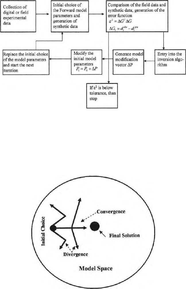
In this chapter a few basic p oints about inversion of geophysical data are given.

Structures of diﬀerent approaches for inversion, viz, Singul ar Value Decompo-

sition, Lea st Squares including Ridge Regression, and Weighted Ridge Regre s-

sion, Minimum Norm Algorithm, Bachus Gilbert Inversion, Stochastic Inver-

sion, Occam’s Inversion Global Optimization Techniques including Monte

Carlo Inversion, Simulated Annealing and Genetic Algorithm, Artiﬁcial Neu-

ral Network and Joint inversion are discussed.

17.1 Introducti on

The task of retrieving complete information ab out model parameters from a

complete and precise set of data is inversion. In geophysics, these mo dels are

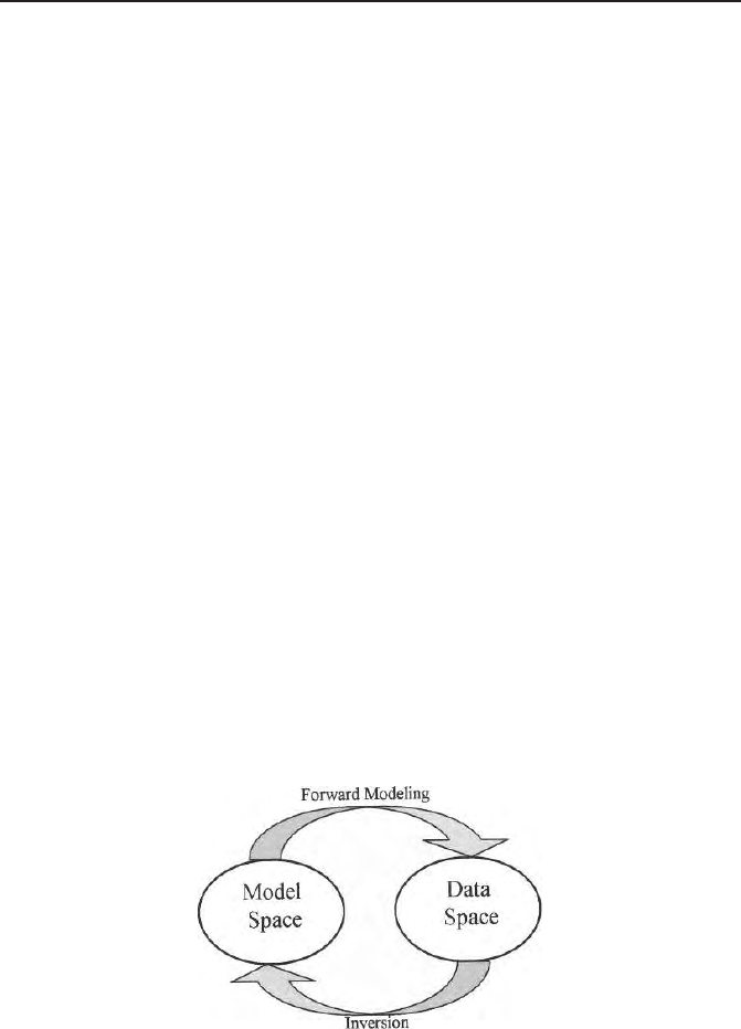
earth models and the task is to establish a link between a data space and

model space (Fig. 17.1).

If we have a set of data collected from the ﬁeld, we try to say about the

earth model with those ﬁnite data set. How many diﬀerent ways can one try

Fig. 17.1. Connecting link between a data and the corresponding model space in

a forward and an inverse problem

562 17 Inversion of Potential Field Data

to travel within a Data space (or domain) and a mo del space (or domain),

how good the ﬂow of information is from a data space to a model space, what

are the diﬃculties can one encounter, how many diﬀerent ways can one try

to overcome those diﬃculties, how much information can one really gather

and what are their limitations, what are the precautions can one take on

the way as one moves through the multidimensional hyperspace (Figs. 17.2

and 17.3) are some of the questions to be addressed brieﬂy. Inverse theory

is applicable to all the branches of science and engineering. Inverse problems

are also termed as identiﬁcation problems or optimization problems. It is

a part of information theory and communication theory. Inverse Theory is

the most scientiﬁc and accurate mathematical tool to be used judiciously for

interpretation of geophysical or other scientiﬁc data.

Some sense of movement, distance and projection of a structure from dif-

ferent angles are involved in an inverse problem. Data and model spaces are

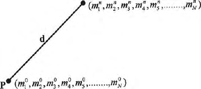
assumed to be n and m-dimensional abstract spaces (Figs. 17.2 and 17.3)

where information from the data space are transmitted to the model space

and vice versa through some connecting links. We shall discuss on these links

in the text. Figure 17.2 show the distance between the starting and the end

point in an m dimensional hyperspace. This sense of distance and movement

are present both in the data and model space. These distances are d

obs

–

predicted

in the data space and m

true

–m

prior

in the model space. We try

to minimize these distances in both the spaces. It means that the model

with which we started our experiment has certain co-ordinates in the abstract

space. That m-dimensional co-ordinate point moves towards the actual answer

as the inverse process progresses. This is the sense of movement in an inverse

problem. These movements can b e continuous in small discrete steps or it

can b e by random jumps in the entire parameter space. What is really meant

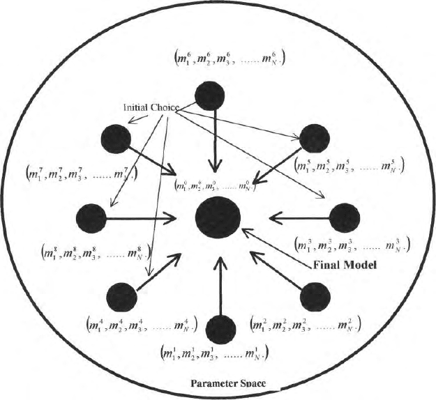
by this movement? Here comes the concept of forward modeling. Figure 17.3

shows the diﬀerent initial choices of the model parameters at diﬀere nt places

in the m-domain but all the movement from the starting points are towards

the actual answer. An initial and judicious choice of a model is the starting

point of an inverse problem. For existence of an inverse problem, the forward

problem must exist. Therefore, solution of a forward problem is the starting

Fig. 17.2. Movement of an assumed model and the sense of distance in an N

dimensional mo del space

17.1 Introduction 563

Fig. 17.3. Diﬀerent initial choices and in M dimensional parameter space and their

movements towards the actual answer

point of an inverse problem. Geophysicists collect a set of data on the surface

of the earth or in the air or inside a bore hole or at the ocean b ottom.What

can we say about the earth with these limited noisy data? That’s how, ‘norm’,

conver gence, metric space, inner product space, Hilbert space n-dimensional

vector space entered in an inverse problem. Figure 17.2 shows the distance

between the actual answer and the starting point.

Generally gravity / magnetic / D.C. resistively / electromagnetic / S.P. /

I.P / Seismic reﬂection a nd refraction / earthquake Seismology / heat ﬂow

data are collected. Interpreters of data have to guess judiciously at this stage

on what kind of subsurface structure can generate this kind of data distribu-

tion. Interpreters must have some insight about the nature of distributio n of

data for diﬀerent type of subsurface structures as well as for diﬀerent types of

potential and non potential ﬁelds. Judicious choice of an initial model reduces

the distance between m

prior

and m

true

where these points are locations of

a priori or initial choice of the model parameters in an abstract space. To

achieve this insight one has to solve mathematical boundary value problems

for diﬀerent types of naturally occurring or artiﬁcial man made ﬁeld s and

564 17 Inversion of Potential Field Data

examine the nature of responses responsible for diﬀerent types of sub surface

structures. These boundary value problems are forward problems and can be

one / two / or three-dimensional problems. With increase in complexity in

an assumed earth model, the mathematical complications in the solution of

a forward problem incre ases. Advent of numerical methods, viz., ﬁ n i te dif-

ference, ﬁnite element, integral equation, volume integral, transmission line,

hybrids, increased the horizon of solvability of the problems of complex sub-

surface g eometry and that incr eased the horizon of applicability of inverse

problems. For the last seven decades, geophysicists solved numerous forward

boundary value problems needed for interpretation of geophysical data. Hence

inversion of geophysical data grew as a subject at a faster pace. The data we

generate by solution o f boundary value problem are noise free synthetic data

obtained from a synthetic model. These synthetic data are called d

Predicted

or d

Pre

and a synthetic model is m

Prior

.Ingeophysicsd

Observed

or d

Obvs

are

generally the ﬁeld data collected on the surface of the earth or in the air or in

o cean surface or in a borehole. These are experimental data in other branch

of science and engineering and are contaminated with noise. (d

Obs

–d

Pre

)

and (m

true

–m

Prior

) are the two distances or norms we were talking about

and we try to minimize these distances in the data s pace and model space

by dual minimization simultaneously. Inverse theory is based o n a few basic

concepts(Parker 1977) viz., (i) existence (ii) construction (iii) approximations

(iv) stability and (v) nonuniqueness.

Existence : For existence of an inverse problem, forward problem must

exist The solution of a boundary value problem is either available or it is to be

solved. Solutions of forward models in analytical form are available (already

solved) for simpler sub surface geometries. With the introduction of realistic

touches in earth models, a boundary value pro blem becomes mathematically

unmanageable and one has to solve the problems numerically.

So the forward problem must be solved or at least must be available before

construction of an inverse problem. Since the model space and data space a re

respectively the Hilbert space and Euclidean space, the concept of projection

of models from diﬀerent angles appear. With limited data and with limited

resolving p ower of many of the potential p roblems we can only see a projection

of the model from a particular angle. That invites a serious problem of non

uniqueness to be taken up.

Construction : Construction of a n inverse problem can be done in many

ways. It is centered around (i) examination of data and to take decision on

application of regularization (ii) judicious assumption of an initial model based

on the nature of the data (iii) solution of the forward problem (iv) comparison

of ﬁeld data with the synthetic model data or predicted data (v) estimation of

the discrepancies (d

obs

–d

pre

) in data space and (m

est

–m

prior

) in the model

space quantitatively in the form of squared residuals or chi square errors or

residual variance or energy function or cost function or error function etc.

(vi) choose a particular type of inversion approach based either on linearised

inversion approach or random walk technique for global optimization approach

17.1 Introduction 565

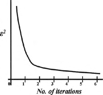
Fig. 17.4. Convergence of an inverse problem in successive iterations

(vi) obtain the convergence of an iterative solutions (Fig. 17.4). (vii) ﬁnd

out the uncertainly l evel in parameter estimation (ix) study the level of non

uniqueness and ﬁnd out the way to overcome it if possible (x) mix some

additional information from diﬀerent branches of geophysics if available and

trytogoforjointinversion.

Multi domain geophysical data based on diﬀerent physical properties can be

used either for joint inversion or these additional information can be used to

constrain the model to be estimated. Some of the very well known approaches

for construction of an inverse problems are (i) Singular value decomposition

(ii) Least squares estimator (iii) Ridge regression and weighted ridge regression

estimators (iv) Min imum norm estimator for an underdetermined problem

(v) Method of steepest descent (vi) Conjugate gradient minimization (vii)

Bachus Gilbert inversion (viii) Stochastic inversion. (ix) Occa m’s inversion.

(x) Monte Carlo inversion (xi) Simulated Annealing (xii) Genetic Algorithm

(xiii) Neural network etc. This is a broad outline about the construction of

an inverse problem. There are many other approaches not listed here.

Figure 17.5 shows a schematic diagram regarding construction of some of

the inversion procedures. Procedural details are diﬀerent for diﬀerent inversion

approaches. Figure 17.6 shows the paths for convergence and divergence in the

parameter space starting from the initial choice.

Approximation is a major component in framing an inverse problem.

Approximation enters into the system throug h many channels. As for exam-

ples most of the geophysical problems are non-linear problems. We linearise

the non-l in ear problems by trun cating higher order terms of the Taylor’s series

expansion and introduce approximation to enter into the domain of general-

ized linear inverse problems. The eﬀect of this truncation of higher order

terms may be less for certain problems. They are called weakly non-linear or

linearisable problems. Fo r certain other cases the eﬀect of linearization may

566 17 Inversion of Potential Field Data

Fig. 17.5. A cartoon of a ﬂow chart for an inverse problem

be severe. They are called strongly non-linear problems. Some of these non-

linear prob lems can be linearised at the maximum likelihood point (discussed

later) whereas some other problems cannot be linearised at all. Therefore,

for strongly nonlinear problems one should use one of the global optimiza-

tion approaches. The next major approximation enters through the choice of

Fig. 17.6. Convergence and divergence of an inverse problem as the initial model

starts moving towards the actual answer

17.1 Introduction 567

forwar d problems. E arth structure is much more complicated than whatever

forward model we choose to initiate an inverse process. The approximation

in very severe for one dimensional modeling and inversion. Only for a few

cases we g et perfect horizontal layers inside the earth. Although numerical

approaches for forward modeling viz. ﬁnite element and ﬁnite diﬀerence can

take care of a part of the degree of complications inside the earth in 2-D/3-

D forward problems, it cannot be a complete substitute for an earth model.

The interpreter must have a reasonable knowledge about the geology of the

area for proper selection of an earth model. A model widely oﬀ from the

actual earth’s subsurface will generate wrong answer even if one gets rea-

sonably good convergence of an inverse pr oblem. Approximations also enter

through data inadequacy, data smoothing and applications of several con-

straints. Some kinds of regularization, viz, Tikhnov’s regularization (Tikhnov

and Arsenin 1977), Occam’s rajor (Constable et al 1987), minimum structure

algorithm (Smith and Booker, 1991) are necessary. Data smoothing is very

common before inversion unless the data are of very high quality.

Stability of an inverse problem means smooth and trouble free move-

ment of all the parameters of a particular model towards the actual answer

and should reach nearer to the destination (Fig. 17.6). For movement from

the initial choice point in the Hilbert space, the inverse problem may start

diverging out. It means the discrepancy between the ﬁeld and predicted data

and the distance b etween model values and the actual answer will also start

increasing, i.e., sum of the squared residual will start increasing instead of

decreasing. Larger the number of parameters in a model space greater will

be the probability for divergence. In the parameter space all the parameters

must move towards the actual answer. In that case the inverse problem is

stable. There are a few reasons f or an inverse problem to be unstable. These

are (i) data inadequacy (ii) data inaccuracy (iii) poor initial choice of the

model parameters (iv) generation of ill conditioned matrix with several zeros

or very small eigen values for the problems dealing with generalized inverse (v)

unconstrained optimization. Presence of several loca l minimum pockets will

not allow the system to converge. The data space and model space are con-

nected by a linear or a linear diﬀerenti al operator. Since most of the geophysi-

cal problems are nonlinear, linear diﬀerential op erators are generally used and

they construct the sensitivity matrix. If the matrix thus generated is an well

conditioned matrix, then with adequate good quality data one can generate

a well posed problem.

In an well posed problem if one gives a small perturbation in the model

parameters, small perturbation in the data space will result and vice versa.

On the other hand if a small perturbation in the data space causes large

perturbation in the model space, then the problem is an ill posed problem.

Most of the geophysical problems are ill posed problems. Zero and small eigen

values of the sensitivity matrix bring this instability. To improve stability of an

inverse problem quite a few steps are taken viz. (i) an attempt is being made

to make the problem overdetermined. An over determined problems are those

568 17 Inversion of Potential Field Data

where the number of data points (n) are more than the number of unknown

parameters (m). n greater than m does not guarantee that the problem will be

an overdetermined problems. Data must b e capable of seeing the entire earth

model within its power of detectibility. For most of the geophysical problems

it becomes possible to collect more data than the number of parameters to be

resolved from the model.

For certain geophysical problems, it may not b e possible to collect as many

data as practicable and the problem becomes underdetermined problem i.e.,

the number of data points is less than the number of unknowns parameters

(n < m). Theoretically or mathematically when n = m, we have an even

determined problem and one should be able to determine m completely. But

presence of noise in ﬁeld data makes the system unstable and the problem

diverges. (ii) detailed eigen value analysis is done to study the rank deﬁciency

of the sensitivity matrix and to weed out the zero and small eigen values (iii)

Marquardt Levenberg co eﬃcients or parameter variance covariance values are

added to the diagonal elements of the sensitivity matrix to ensure stability

(iv) Positivity or non negativity constraints are imp osed for not allowing any

of the parameter to be negative when it is known that the parameters to

be determined are deﬁnitely positive quantities. Constraints on upper and

lower bounds of a particular parameter can also be introduced. Constraints

on movement in the parameter space is also introduced to ensure b etter sta-

bility (v) introduction of a prior assumption from reliable other geophysical or

geological data may reduce the number of unknown parameters to be deter-

mined and thereby improve the stability condition and quality of inversion to

a certain extent.

Nonuniquenesses are very imp o rtant aspects of an inverse problem to be

taken care of. If we have or assume a model we can generate a unique respo n se

for a particular type of ﬁeld. But the reverse is not true, i.e., if we have a s et

of data, inﬁnitely many models may satisfy this set of data It is possible to

overcome this hopeless situation to a great extent and that is why the inverse

theory survived the test of time. The causes for the non uniqueness in an

inverse problem are as follows:

Nonuniqueness is due to (i) principle of ambiguity present in the potential

theory (ii) data inadequacy (iii) data inaccuracy, (iv) diﬀerent form of error

present in the data (v) noise (vi) bad initial choice of the model parameters,

(vii) diﬀerent types of constraints imposed, (viii) presence of several local

minima pockets in the parameter space (Figs. 17.7 a, b) (ix) simpliﬁcation of

the forward model, (x) linearization of the nonlinear problem, (xi) diﬀerent

approaches are adapted for solution of inverse problems, (xii) diﬀerent types

of corrections applied to the data, (xiii) various types of smoothing applied

to the data. (xiv) diﬀerent forward problem soft wares used to interpret same

data.

Green’s theorem of equivalent layer s in potential theory discussed in

Chap. 10 is an example of n on uniqueness present in theory. This theorem

shows that one can get same gravitational ﬁeld for diﬀerent type of mass