Roy K.K. Potential theory in applied geophysics

Подождите немного. Документ загружается.

17.11 Minimum Norm Algorithm for an Under Determined Problem 589

f=ε

−1

ε =(y− xβ)

−1

(y − xβ)

=∆G

−1

∆G

. (17.117)

When the observations are independent and the errors are uncorrelated, all

the covariance terms will be zero and the variance – covariance matrix will

simply be a diagonal matrix.

Therefore the weighted least squares estimator can be written as

∧

∆P =



−1



−1

∆G (17.118)

and weighted ridge regressions estimator can be written as

∧

∆P

∗



−1

X+K I



−1

∆G. (17.119)

Here the data are weighted by the inverse square root of the data variance-

covariance matrix. (Inman, 1975).

The covariance matrix is given by

V=σ



−1



−1

(17.120)

where

∆G

−1

∆G

n − m

. (17.121)

Here σ

is termed as the residual variance and n and m are respectively

the number of data points and number of parameters to be retrieved. The

parameter standard error or the parameter uncertainly is deﬁned as the square

ro ot of the diagonal elements of the parameter variance-covariance matrix.

Thus

√

......... etc. the parameter uncertainties are added to the

retrieved model parameters i.e., the estimated parameters will now be written













, .....etc.

Data variance covariance matrix W is assumed to be a diagonal variance

matrix with zero or negligible oﬀ diagonal covariance part.Reciprocals o f the

standard deviations are data weights and is given by

W=(1/σ

, 1/σ

, ·······························1/σ

)

where variance is square of standard deviation.

17.11 Minimum Norm Algorithm for an Under

Determined Problem

17.11.1 Norm

Norm i s a measur e of distance or length i.e., the distance between d

Obs

and

Pre

or m

Prior

and m

true

. For each observations, one deﬁnes a predictable error

or misﬁt

590 17 Inversion of Potential Field Data

Obs

− d

Pr e

The best line is the one with smallest over all error E.



i=1

This exactly is the squared Euclidean length. In the parameter domain L =

i=1

= m

m. Here E and L are respectively the square of sum of the

lengths in the data and parameter domains. Here m

= m

true

− m

Pr ior

for

the ith parameter. The norm is indicated by double bar i.e., E = e.The

-----------L

norms are deﬁned as

1 norm

= e

)



i=1

|e|

(17.122)

2norm

= e

)



i=1

1/2

(17.123)

nnorm

= e

)



i=1

1/n

(17.124)

∞ norm

= e

∞

=max|e

| (17.125)

Successive higher norms give larger weightage to the largest element of e.

Therefore L

∞

norm is the highest value of e

17.11.2 Minimum Norm Estimator

William Menke (1984) discussed this algorithm fo r solving underdetermined

problems using Lagrange multipliers. Underdetermined problems are those

where the number of data points are less than the number of unknown param-

eters to be determined. Underdetermined problems have generally inﬁnite

number of solutions. It is diﬃcult to ch oose the correct one out of many. That

is why some additional information k nown as a priori information are neces-

sary to interprete an underdetermined inverse problem. Lagrange multipliers

maximizes or minimizes a certain function using a constraint equation.

Here in this problem we have to ﬁnd a model m

estimated

or m

est

that

minimizes

L = m

m =



(17.126)

subject to the constraint equation that e = d − Gm = 0

where e is the error. The inverse problem is d = Gm. This problem can be

solved using Lagrange multiplier. We can minimize the function

17.11 Minimum Norm Algorithm for an Under Determined Problem 591

φ (m) = L +



i=1

(17.127)

φ (m)=L +



i=1



i=1



i=1

)

−



J=1

(17.128)

where λ

is the Lagrange multiplier, G

is the frechet kernel. Taking the

derivations with respect to m

,weget

∂φ

∂m



i=1

∂m

−



i=1



j=1

∂m

(17.129)

=2m

−



i=1

. (17.130)

Taking

∂φ

∂m

=0,

we get

2m = G

λ (17.131)

in matrix notation. Taking the constraint equation Gm = d, and substituting

this equation in (17.101), we g et

d=Gm=G(G

λ/2). (17.132)

The matrix GG

is an N×N matrix. If its inverse exists then we get the value

of the Lagrange multiplier as

λ =2





−1

d. (17.133)

The expression for the minimum norm estimator for an under determin ed

problem is

est





−1

−g

d. (17.134)

−g

is a generalized inverse for an under determined problem. Whatever pre-

scriptions are made for least squares estimator for an over determined problem

regar d in g use of Marquardt’s coeﬃcient to handle zero and very small eigen

values of the system matrix are also valid for under determined problems. The

least squares and minimum norm generalized inverses are respectively given

−g





−1

(Least Squares) (17.135)

and

592 17 Inversion of Potential Field Data

−g





−1

(Minimum norm) (17.136)

Generalized inverse gives m

estimated

or m

est

−g

obs

from d = Gm. There-

fore we can write d

Pre

=Gm

est

=G(G

−g

obs

)=(GG

−g

obs

=Nd

obs

. (17.137)

The n × n square matrix N = GG

−g

is called the data resolution matrix.

The diagonal elements of this matrix give a quantitative idea about the data

importance.

Data importance n = diag(N).

Similarly model resolution matrix

est

−g

obs

−g

true

(

(17.138)

−g

(

true

=Rm

true

. (17.139)

Here R is m × m model resolution matrix. If R = 1 , then ea ch model is we ll

determined. Like N, it is also a diagonally dominant matrix.

Information density matrix uu

and resolution matrix vv

has

some similarity with N and R respectively. But the values do not come exactly

same. uu

and N = GG

−g

are in data space, vv

and R = G

−g

are in the model space.

Dirichlet’s spread functions are deﬁned as

Spread = (N) = N −I =



i=1



j=1

− I

]

(17.140)

Spread = (R) = N −I =



i=1



j=1

− I

]

. (17.141)

The spread qualitatively indicates the quality of inversion. Large r the spread

worse will be the inverted model. n and m are respectively the number of data

points and number of parameters. I is the identity matrix therefore I

=0.

17.12 Bachus – Gilbert Inversion

17.12.1 Intro du ction

Bachus – Gilbert theory of inversion isalsoamemberofthelinearinverse

theory. But the approach is signiﬁcantly diﬀerent from those we have discussed

so far. Here we describe and apply a method of ﬁnding the resolving power of

a ﬁnite set of data when these data are used to construct an earth model.

Bachus – Gilbert’s theory say that if we can construct an inverse problem

such that when we try to ﬁnd out the physical property of the earth at a

17.12 Bachus – Gilbert Inversion 593

depth z

say (m)

, then the mathematical system should pickup maximum

information from that depth z

and very little information from above and

below that depth. In other words if we can construct a ke rnel which have dirac

delta type behaviour, then only it will be possible to pick up in formation

only from one depth. With ﬁnite numb er of data, it is not possible to get

such a sharp dirac delta type kernel. B-G named this kernel as an averaging

kernel A(z, z

). It not only picks up information from that depth z

but also

carries some information from depths ab ove and below. This averaging kernel

has certain width or spread. Lower the spread, sharper will be the pick of

the averaging kernel. B-G made the mathematical formulation in such a way

that they tried to minimize the spread using Lagrange multiplier and using

the constraint equation. i.e., the area under the averaging kernel in equal to

unity. So the deltaness criterion of the averaging kernel and minimization of

the spread function go together at all depths and the model parameter m

is determined. Gradual increase of the B-G spread function with depth will

roughly tell about the depth upto which the earth model could be estimated

with a certain degree of certainty using a ﬁnite number of data.

17.12.2 B-G Formulation

The imp ortant advantages of the B-G method are (i) layered earth approx-

imation is not required. The physical property say resistivity o r density is

a function of the depth z only i.e. ρ =f(z)atthepointofmeasurement.

Therefore data collected over a complicated Archean-Proterozoic geological

terrain can also be inverted using B-G a p p roach (ii) depth of explor ation of

the D.C resistivity, electromagnetic and magnetotelluric sounding data can

be estimated from B-G spread function.

B-G assumed that the earth functionals are linear and they are fre’che’t

diﬀerentiable. Therefore the linear earth functionals g

,......g

(ﬁeld

data) can be connected to the earth model parameter through the Fredhom’s

integral of the ﬁrst kind i.e.

(m) =



(z) m (z) dz (17.142)

where G

(z) is a known function of z because g is a known linear functional.

So the inverse problem is what can we say about m(z) at z = z

when all

we know is a set of g

,......g

collected on the surface of the earth. We

try to compute m

which is the average value of m taken within a short

interval z

± ∆z

. These local averages are the model value at a particular

depth z

within the resolving length z

+∆z

to z

− ∆z

. B-G deﬁned the

local average using the averaging kernel in the form

m

zmax



A(z

, z) m (z) dz (17.143)

594 17 Inversion of Potential Field Data

where averaging kernel assumed to be unimodular and it is

zmax



A(z

, z) dz = 1. (17.144)

The averaging kernel A is distributed in z i.e., at depths where we shall try

to compute m(z), we shall have to compute the averaging kernel to examine

the quality of inversion based on the strength of the data. Data quality and

adequacy improves the quality of A. Theoretically the nature of A should be

unimodular, for practical probl ems when the data contains noise, A can show

multimodular nature and spread may incr ease very fast. Ideally A (z

, z) =

δ(z − z

)whereδ is the Dirac delta distribution. With only a ﬁnite number

of ﬁeld data, available for computing m

, we should not expect the local

average to be so localized.

We assume that the average m

, whatever it turns out to be, depends

only on g

(m), g

(m) ......g

(m).

Since m

and g

(m), g

(m) ......g

(m) have linear relation, we can

write

m



i=1

(m) (17.145)

These coeﬃcients depends on the depth z

. At each depth we have to ﬁnd out

these coeﬃcients a

)toestimatem

and the additional constraint is

A(z

, z) =



i=1

(z) . (17.146)

So we have to determine the a

) at all depths such that it satisﬁes (17.143)

(17.144) (17.145). B-G chose a function K (z

, z) which vanishes at z = z

and

increases on b oth the sides of z

. B-G chose the function

K=12

∞



(z − z

)

(z, z

)dz. (17.147)

Here the factor 12 in (17.147) is used so that the spread b ecomes equal to

width of the averaging kernel. We can write the value of K from (17.147) and

(17.146) in the form



i=1



j=1

⎧

⎨

⎩

∞



(z −z

)

(z) G

(z) dz

⎫

⎬

⎭

(17.148)



i=1



j=1

. (17.149)

17.12 Bachus – Gilbert Inversion 595

In the matrix form

K=a

S a (17.150)

where S = S

K is interpreted as the spread around z

(Oldenburg 1979). The matrix S is

called the spread matrix. The elements of matrix S can be written i n simpler

computational form as

=12

∞



(z − z

)

(z) G

(z) dz (17.151)

⎡

⎣

∞



(z) G

(z) dz

⎤

⎦

− 2z

⎡

⎣

∞



(z) G

(z) dz

⎤

⎦

⎡

⎣

∞



(z) G

(z) dz

⎤

⎦

. (17.152)

The construction of the averaging Kernel requires computation of averaging

coeﬃcients a

), (i = 1, 2,.........N) around the depth of interest. These

coeﬃcients are determined minimizing the spread using Lagrange multiplier

and using the constraint i.e., the area under the averaging kernel is equal to

unity. We can write (17.148) in the form



i=1

∞



(z) dz = 1 (17.153)

⇒



i=1

= 1 (17.154)

where

∞



(z) dz. (17.155)

Andinthematrixformwecanwrite

⇒ a

u=1. (17.156)

The minimization of ‘a

S a’ under the constraint a

u = 1 using Lagrange

multiplier technique solves the problem of determining coeﬃcients of the aver-

aging kernel. Applying this technique, the condition for minimization of the

spread with respect to a is

∂

∂a

)



i=1



J=1

− λ

′





− 1



= 0 (17.157)

596 17 Inversion of Potential Field Data

where λ

′

is the Lagrange multiplier

and when i = j, a

and

∂

∂a

=2a

. Therefore



j=1

− λ

′

= 0 (17.158)

where

λ =

′

In the matrix form

Sa− λ u=0

⇒ a=λ S

−1

u. (17.159)

Since

u=1

⇒ λ u

−1

u=1

⇒ λ =

−1

. (17.160)

Hence

a=S

−1

u/(u

−1

u). (17.161)

Equations (17.159) and (17.161) shows respectively the values of the Lagrange

multipliers and the coeﬃcients of the averaging kernel which minimizes the

spread. The corresponding model estimate is given by

m

−1

(17.162)

and the averaging kernel is determined as

A(z, z

G(z)

−1

. (17.163)

Thus all the parameters of B-G inversion are obtained. But one problem is

yet to be solved i.e. how to determine the fre’che’t kernel G (z). Oldenburg

(1978 and 1979) have shown the procedure for determination of G (z) for

d.c resistivity and magnetotelluric inversion applying B-G method. In the

presence of noise, the s pread matrix ‘S’ is replaced by W in the form.

W=(1− α)S + α Cov (m). (17.164)

Here error in the model estimate is related to the error in the data. The

variance in the estimated model is considered as a measure of error. Covariance

17.13 Stochastic Inversion 597

matrix is constructed and a fraction of that is taken in the modiﬁed spr ead.

α is a fraction. It varies from 0 to 1. For very good quality data α =0,

and W = S. With increase in noise α increases. α = 1 for totally noisy

data. The averaging coeﬃcients are obtained by minimizing a

Wainsteadof

S a. The coeﬃcients thus obtained are the functions of α. The procedure

for minimizing W is the same as that for S. A trade oﬀ between resolution

and the variance-covariance is made for optimum choice of α.

In B-G inversion no initial choice of the model parameter is necessary.

Therefore it can be used for any kind of complicated geology. Any physical

property is assumed to be just a function of depth. One can see the strength of

the data and the quality of inversion from the nature of the averaging kernel.

One can directly see the depth of investigation of the data. Beyond a certain

depth, the B-G spread function explodes i.e., the spreads start increasing at

a very faster rate. That dictates the depth upto which the data could see the

subsurface.

17.13 Stochastic Inversion

17.13.1 Intro du ction

In this inversion approach most of the basic ingradients of inversion are

viewed from the angle of probility density functions although it is basically

a dual minimization approach. Instead of minimizing the error function in

successive iteration we maximize the probability density function assum-

ing Gaussian distribution for linear and linearisable problems. Some of the

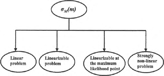
ideas o f Tarantola (1987) are described very brieﬂy. Four classes of problems

(Fig. 17.10) viz, linear, linearisable, nonlinear but linearisable at the maximum

Fig. 17.10. Four classes of an inverse problems (a) linear (b) non linear but linearis-

able (c) nonlinear but linearisable at the maximum likelihood point (d) nonlinear

and not linearisable

598 17 Inversion of Potential Field Data

likelihood point and strongly nonlinear problems and three classes of prob-

ability density functions viz, joint probability density function, conditional

probability density function and marginal probability density function are

used (Freund and Walpole,1987). Since most of the geophysical problems are

nonlinear we work mostly with last three classes of problems. It has already

been mentioned that one linearises a nonlinear problem by truncating higher

order terms of the Taylor’s series expansion. The quantum of error present in

this approximation dictates the degree of nonlinearity of a problem. Higher

the degree of nonlinearity more will be the deviation of the nature of the prob-

ability density function from the Gaussian nature. In the stochastic domain

the existence of an inverse problem is connected with the existence of marginal

probability density function. Here there are more of mixing of information in

the (D × M) parameter space collected from the data (D) and Model (M)

spaces.

Errors due to modeling, instrumentation is expressed in the form of joint

probability density – functions θ(d, m) and ρ(d, m). Here ‘d’ stands for data

and m stands for model. ρ(d, m) is a mixture of information from ρ(d) and

ρ(m) where ρ(d) is the probability density function due to the data error

obs

− d

Pre

)andρ(m) is the probability density function due to modeling

error (m

Prior

−m

true

). These probabilities are described in the form of Gaus-

sion distribution. These probabilit ies are combined to form a joint probability

density function. σ(d, m). It is the starting point of stochastic inv e rsion. From

σ(d, m), we ﬁnd out the marginal probability density functions σ

(m) in the

model space and σ

(d) in the data apace. Since geophysicists are mostly inter-

ested to get models from a set of data, therefore, we are interested in σ

(m),

the marginal probability density function in the model space. It extracts all

information about the model from the joint a posteriori probability density

function σ(d, m). Figure 17.11 is a curtoon of stochastic inversion scheme.

Error due to modeling will always exist. We shall never be able to choo se an

earth model which will exactly match with the reality. In general the chosen

model will always be much simpler than the rea l earth where the data are

collected. So there will always b e some diﬀerence between d

Pre

and d

Obs

.Even

when we get d

Obs

≈ d

Pre

in an iterative process there is no guarantee that we

obtained all the subsurface features in the earth model and in fact we retrieve

a much simpler model. E rror due to instr umentation was severe in earlier days.

With sophistication in instrumentation in modern day digital electronics, error

due to instrumentation has signiﬁcantly gone down. Tarantola expressed these

uncertainties in modeling in the form of Gaussian probability density function

θ (d |m )=



(2π)

det (C

(m))



−1/2

∗

exp



−

(d −g (m))

−1

(m)(d − g (m))



(17.165)

Here d

Pre

Cal

= g (m). For linear inverse problem we have shown already

that we li nearise at the reference point as