Roy K.K. Potential theory in applied geophysics

Подождите немного. Документ загружается.

15.7 Finite Element Formulation Galerkin’s Approach Magnetotellurics 509

[A].[φ]=[S]. (15.115)

For a 3-D problem with tetrahedral elements,the matrix A will be a hepta

diagonal,diagonally dominant sparse symmetric matrix.Suitable matrix solver

may be used to obtain φ at all the nodes.

15.7 Finite Element Formulation Galerkin’s Approach

Magnetotellurics

15.7.1 Introduction

Coggon (1971), Silvester and Heslam (1972), Rodi (1975), Pelton et al (1978),

Wannamaker (1984, 1987), Kikkonen (1977) did mathematical formulaton on

ﬁnite element method for geo-electric and geo electromagnetic problems. In

this section we present a brief description of the ﬁnite element method for TE

and TM mode magnetotellurics (Plane wave normal incidence electromagnet-

ics). The ﬁnite element approach for solution of the Helmoltz wave equation

is presented.

Let us consider TE mode MT in which E

= ∂/∂y=0.For

harmonic ﬁelds in the case of plane wave electromagnetics, we get

∂E

/∂z=iωµ H

(15.116)

∂E

/∂z=−iωµ H

(15.117)

and

∂H

/∂z − ∂H

/∂x=iωε E

. (15.118)

We get

∂/∂x(1/iωµ ∂E

/∂x) + ∂/∂z(1/iωµ ∂E

/∂z) − iω ∈ E

=0. (15.119)

For TM mode, we get

= ∂/∂y=0

and

∂H

/∂z=−iω ∈ E

(15.120)

∂H

/∂x=iω ∈ E

(15.121)

and

∂E

/∂z − ∂E

/∂x=−iωµ H

. (15.122)

Substituting (15.120) and (15.121) in (15.122), we obtain

∂/∂x(1/iω ∈ ∂H

/∂x) + ∂/∂z(1/iω ∈ ∂H

/∂z) − iωµ H

=0. (15.123)

The general expression for two d imensional Helmoltz equation is

∂/∂x(1/k ∂f/∂x) + ∂/∂y(1/k ∂f/∂y) + p(f) = S. (15.124)

510 15 Numerical Methods in Potential Theory

15.7.2 Finite Element Formulation for Helmholtz Wave Equations

This ﬁnite element formulation is based on the work of Wannamaker (1984,

1986 and 1987) The ﬁnite element formulation is constructed as follows:

(a) The region is divided into ﬁnite number of sub-domains selected here as

triangular elements. These elements are connected at common node points

and collectively form the shape o f the region.

(b) The continuous unknown function ‘f’ is approximated over each element

by polynomials selected here as lin ear polynomia ls. These polynomials are

deﬁned using the noded values of the continuous function ‘f’. The value

of a continuous function ‘f’ at each nodal point is denoted as a variable

which is to be determined.

the Helmholtz equation using linear polynomials.

(d) The regions of application of Neumann and Dirichlet boundary conditions

are established.

(e) Element equations are converted into element matrix equations.

(f) The matrix element equations are assembled to form the global matrix

equations.

(g) The boundary conditions are introduced.

(h) The system of linear equations are solved.

One important aspect of the ﬁnite element method is the design of the dis-

cretized domain i.e. the construction of ﬁnite element mesh. The construction

of the mesh is problem dependent. The working domain is discretized with

ﬁnite elements of diﬀerent 2-D or 3-D shapes depending upon the dimension

of the problem. The size of the mesh must be variable and near the discontinu-

ities the mesh size should be ﬁner. The area where there is no inhomogeneity

the mesh can be coarser. For two dimensional bodies triangular, rectangu-

lar, hexagonal meshes can be used. For 3-D b odies cubical parallelopiped,

tetrahedral elements can be used. Depending upon the nature of complexity

complicated isoparametric elements with 8 nodes, 20 nodes, 32 nodes cubic

elements can be used as shown in the next section. The connecting points of

all the elements are nodes. In the discretized domain we try to ﬁnd out the

ﬁelds or potentials at these nodal points.

In the following section we present the basics of ﬁ nite element formula-

tion for magnetotelluric boundary value problems using triangular elements.

Initial part of the formulation is same as that outlined in the previous sec-

tion. In this section the Galerkins methods is used. So the formulation takes

a diﬀerent path. The elements are triangular, the simplest elements for a two

dimensional problem. The guiding equations are electromagnetic wave equa-

tions and Maxwell’s electromagnetic equations. The boundary conditions are

mentioned in the Sect. 15.4.

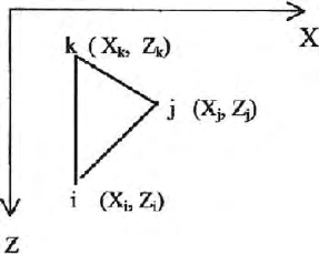
We assume an arbitrary triangular element (e) within the ﬁnite domain

with nodes at the vertices of the triangles (Fig. 15.19).

15.7 Finite Element Formulation Galerkin’s Approach Magnetotellurics 511

Fig. 15.19. Triangular ﬁnite element for MT ﬁeld formulation

With this type of domain discretization we allowed the functional to vary

linearly over each element. The plane passing through the nodal values of ‘f’

attached with each element (e) can be described by the equation:

(x, y) = a

(e)

X+a

(e)

Z. (15.125)

At the three nodes the values of the assumed polynomials are:

(e)

(x, y) = α

(e)

+ α

(e)

+ α

(e)

(15.126)

(e)

(x, y) = α

(e)

+ α

(e)

+ α

(e)

(15.127)

(e)

(x, y) = α

(e)

+ α

(e)

+ α

(e)

We solve these equations for α

, α

and α

and insert these values in (15.125)

to get

(e)

(15.128)

in which

(e)

=1/2∆(a

X+c

Z) (15.129)

where

− x

(15.130)

j−

− x

(15.131)

and ∆ is the area of the triangular element (e). Like wise the terms N

(e)

and

(e)

are obtained through a cyclic permutations of the subscripts i, j and k.

The functions N

(e)

and N

(e)

are called the shape functions, interpolation

function or the basis function.

Equation (15.128) can be expressed as the matrix equation in the form

(e)

. (15.132)

512 15 Numerical Methods in Potential Theory

In which

(e)

=[N

(e)

] (15.133)

and

=[f

(e)

]. (15.134)

If the domain contains M triangular elements, the complete representation

of the unknown function ‘f’ over the whole domain is given by

f(x, z)=



e=1

(x, z)=



e=1

. (15.135)

This is the function ‘f’ deﬁned over whole domain. We shall derive the element

equations.

15.7.3 Element Equations

The domain equation may be written in the concise form as

L f = s (15.136)

In which

L =

∂

∂x



∂

∂x



∂

∂y



∂

∂y



+ P (15.137)

Inserting the approximate value of f(x, z) given by (15.136) and (15.137) we

get



(e)

) − s=ε (15.138)

in which ε is the residual error to be minimized. Our way to accomplish this

objective is to use the inner product or dot-product between the error vector

and the function. The dot product becomes zero when they are orthogonal or

,ε>=



(e)

εdxdz = 0 (15.139)

for each of the basis function N

(e)

. This integral mathematically states that

the basis function must be orthogonal to the error over the element (e). This

is Galerkin’s method.

Using (15.136) to (15.139), we can write



(e)

[

∂

∂x

(

∂f

∂x

)] + Pf

(e)

− s]dxdz = 0 (15.140)

in which (e) is the triangular region and n = i, jandk.

Applying integration by parts, we get

15.7 Finite Element Formulation Galerkin’s Approach Magnetotellurics 513



(e)

∂

∂x

(

∂f

(e)

∂x

)dxdz = −



∂f

(e)

∂x

∂N

(e)

∂x

dxdz +



∂f

(e)

∂x

(e)

(15.141a)

in which n

is the x-component of the unit normal to the boundary, dl is a

diﬀerential arc length along the boundary. When we treat the second term in

(15.140) in the same manner, the (15.140) takes the form



(e)

[−

(

∂f

(e)

∂x

∂N

∂x

−

∂f

(e)

∂z

∂N

(e)

∂z

)+N

(Pf

(e)

− s)]dxdz



∂f

(e)

∂n

(e)

dl = 0 (15.141b)

in which

∂f

(e)

∂n

∂f

(e)

∂x

∂f

(e)

∂z

. (15.142)

With the surface integral in (15.141b) and selected boundary conditions, we

can write (15.141b) using (15.140,15.141a)



−

(

∂N

(e)

∂x

∂N

(e)

∂x

∂N

(e)

∂z

∂N

(e)

∂z

)dxdz +



(e)

dxdz

−



(e)

dxdz = 0 (15.143)

in which n = i, j, k. We can rewrite (15.143) in the matrix form as

(e)

+ P

(e)

= S

(e)

(15.144)

in which the matrices K

(e)

and vector S

(e)

have the entities

= −



(e)

(

∂N

∂x

∂N

∂x

∂N

∂z

∂N

∂z

)dxdz (15.145)



(e)

dxdz (15.146)

and



dxdz. (15.147)

Assuming K and P to be constant within the element e and using (15.144) to

(15.146) and the integral

514 15 Numerical Methods in Potential Theory



(e)

dxdz =

2a!b!c!∆

(a + b + c +2)!

(15.148)

in which ∆ is the area of the element, we may write (15.134) to (15.145) as

−

4k∆

⎡

⎣

+ c

⎤

⎦

P ∆

⎡

⎣

211

121

112

⎤

⎦

(e)

+ S

(e)

=0. (15.149)

It is interesting to note that (15.149) is applicable for MT, DC resistivity, EM

etc. , but source term will be diﬀerent in diﬀerent problems. Imposition of

boundary condition will also be diﬀerent for diﬀerent problems. For magne-

totelluric problem S

(e)

is identically zero.

Equation (15.149) is known as element matrix equation for the triangular

element (e). For each element in the domain an equation of the form (15.148)

can be derived. These equations can be assembled (summed) into a single

matrix equation. Details of the assemblage of the global matrix equation ar e

discussed in the Sect. 15.5 and given in Zienkiewicz (1971). The global matrix

equation can be written as

Gf = S (15.150)

where G is a N×N symmetric, sparse, banded and diagonally dominant matrix

and N is the total number of nodal points in the entire discretized domain.

The vector f is a column vector of N unknown values of the function f (x, z)

at each node of the model. The vector S is a column vector that contains the

source information given by adding the contribution of all the source terms

(e)

αI

360

⎡

⎣

⎤

⎦

(15.151)

where α is the angle subtended by element e. I is the current strength. It is

applicable for DC resistivity and not for MT. For the global matrix, all the

boundary conditions dema nd ed by the problem must be introduced ﬁrst and

then the matrix equation is solved using one of the suitable matrix solver viz.,

(i) Gauss Elimination (ii) Gauss-Siedel Iteration (iii) Cholesky’s Decomposi-

tion (iv) Conjugate Gradient Minimization etc. Thus the unknown value of

‘f’ i.e. E or H in this case of MT and potential in the case of DC resistivity

at all the nodal points will be obtained. Boundary conditions for MT and DC

resistivity are considerably diﬀerent as discussed already.

15.8 Galerkin’s Approach Isoparametric Elements Magnetotellurics 515

15.8 Finite Element Formulation Galerkin’s Approach

Isoparametric Elements Magnetotellurics

15.8.1 Introduction

In t hi s section a brief presentation on the structure of ﬁnite element formu-

lation using isoparametric elements and Galerkin’s method is given. Since

Galerkin’s method is discussed in the previous section with all it’s essential

details, some of the steps will be avoided while demonstrating the ﬁnite ele-

ment formulation using eight noded isoparametric elements (Murthy 2000).

Basic structure of formulation is based on the work of Wannamaker et al

(1987). All the details about mesh generation, boundary conditions in TE

and TM mode Plane wave electromagnetics , governing diﬀerential equ ations

are given in Sects. 15.4 and 15.7. A few p o ints ab out isoparametric elements

and natural coordinates are added here.

To simulate a complicated and sharp curvatures of a bound ary of a body of

irregular shape, one needs numerous small elements straight edges to reduce

the diﬀerence in shape of the actual and simulated body. Isoparametric ele-

ments can signiﬁcantly reduce the number of elements to be taken because

the elements can take care of curved boundaries of a body very eﬀectively.

These elements are typically meant for bodies of arbitrary shap es. In isopara-

metric domain the coordinates are called natural coordinates and they are

nondimensional. These elements are called isoparametric because the number

of nodes in an element in cartisian coordinate and natural coordinates are

same.

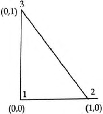
For any variable function Φ within a triangular parent element (simplest

2D element) the prescribed values at the nodes can be obta in ed assuming a

linear polynomial function within the element as

Φ=α

+ α

ξ + α

ζ. (15.152)

In this Fig. (15.20)

Fig. 15.20. A simplest triangular element with natural coordinate

516 15 Numerical Methods in Potential Theory

Since

Φ=Φ

at node 1(ξ =0, ζ =0),

Φ=Φ

at node 2(ξ =1, ζ = 0) (15.153)

Φ=Φ

at node 3(ξ =0, ζ =1),

from (15.153), we get

=Φ

+ α

=Φ

(15.154)

+ α

=Φ

The polynomial coeﬃcients from these equation are

=Φ

− Φ

(15.155)

=Φ

− Φ

Substituting these values, the (15.152) can be written as

Φ=N

(15.156)

where Φ

,Φ

and Φ

are nodal potentials or ﬁelds and N

and N

are

element shape functions. They are connected to the natural coordinates in

isoparametric domain as

=1− ξ −ζ

= ξ (15.157)

= ζ

From (15.154), (15.155), (15.156) and (15.157) we get where

= 1 (15.158)

=0.

Thus we can write the connecting relationship between the cartisian coordi -

nates and the natural coordinates as





i=1

(ξ, ζ)



(15.159)

where X

and Z

are the cartisian coordinates of the ith element. The con-

necting link between the ﬁelds at the centre of a triangle and the nodal values

are

15.8 Galerkin’s Approach Isoparametric Elements Magnetotellurics 517





i=1

(ξ, ζ)



. (15.160)

The cartisian derivatives of the shape function N

in terms of the natural

coordina t es can be written as

∂N

∂ξ

∂N

∂x

∂ξ

∂N

∂z

∂ξ

(15.161)

∂N

∂ζ

∂N

∂x

∂ζ

∂N

∂z

∂ζ

(15.162)

which in matrix form can be written as

⎡

⎢

⎣

∂N

∂ξ

∂N

∂ζ

⎤

⎥

⎦

⎡

⎢

⎣

∂x

∂ξ

∂z

∂ξ

∂x

∂ζ

∂z

∂ζ

⎤

⎥

⎦

⎡

⎢

⎣

∂N

∂x

∂N

∂z

⎤

⎥

⎦

=[J]

⎡

⎢

⎣

∂N

∂x

∂N

∂z

⎤

⎥

⎦

. (15.163)

where J is the Jacobian matrix and can be evaluated using

|J| =



i=1

⎡

⎣

∂N

∂ξ

∂N

∂ξ

∂N

∂ζ

∂N

∂ζ

⎤

⎦

. (15.164)

The derivatives of shape function in Cartisian coor dinate can be obtained in

terms of natural coordinate and can be written as

⎡

⎣

∂N

∂x

∂N

∂ζ

⎤

⎦

=[J]

−1

⎡

⎣

∂N

∂ξ

∂N

∂ζ

⎤

⎦

(15.165)

where the determinant of the Jacobian matrix must be n on zero.

15.8.2 Finite Element Formulation

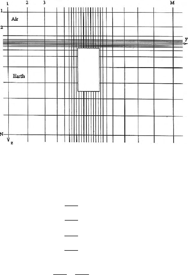
Figure (15.21) shows the typical mesh generated using the quadrilateral ﬁnite

elements. A h omogeneous external region is included in the mesh to facilitate

inclusion of boundary conditions. The resistivity of this region is held ﬁxed at

the average value of the apparent resistivity data. The no dal ﬁeld values at the

bottom and sides of the mesh are set equal to the analytical values obtained

for the homogeneous space. Vertical element dimensions may be increased

approximately exponentially downward from the air-earth interface because

of exponential decay of the ﬁelds. Along the horizontal element boundaries,

we extended the mesh from ﬁne to coarse as we go away from the working

zone. The nodes in the y-direction are indexed by i = 1, 2, 3 ...Mandthe

nodes in the z- d i rections are j = 1, 2, 3 ...N.

Taking the x-axis pa rallel to strike, y-axis in the horizontal and z-axis

positive downward, for the TE mode 2-D geometries, E

∂

∂x

=0.

518 15 Numerical Methods in Potential Theory

Fig. 15.21. A ﬁnite element mesh with quadrilateral boundaries;model shows the

air-earth b oundary and air layers on top of it,the anomalous body and the host

rocks;expanding grid is shown b oth upward,downward ans lateral directions from

the centre of the body

From Maxwell’s equations we can write

∂E

∂z

=ˆzH

(15.166)

∂E

∂y

=ˆzH

(15.167)

∂H

∂z

=ˆyE

+∆ˆyE

(15.168)

∂H

∂y

=ˆyE

+∆ˆyE

(15.169)

and

∂H

∂y

−

∂H

∂z

=ˆyE

+∆ˆyE

(15.170)

(Chaps. 12 and 13 and Table 15.1)) where ˆy = σ + iω ∈ is the admittivit y,

ˆz = iωμ

is the impedivity, ∆ˆy =ˆy

˜ˆy

.whereˆy

and ˆy

indicates the admit-

tivity diﬀerence between the layered host and its 2D inhomogeneity. Subscripts

p and s refer to primary (layered earth) and secondary ﬁeld components.

Substituting (15.166) and (15.167) into (15.168) , the TE mode Helmholtz