Roy K.K. Potential theory in applied geophysics

Подождите немного. Документ загружается.

15.3 Finite Diﬀerence Formulation Domain with Cylindrical Symmetry 489

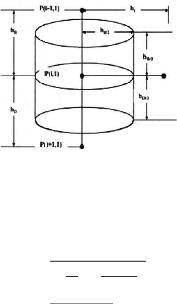
Fig. 15.10. An elementary volume near the point current electrode. On the axis of

a borehole

point source P

(1,1)

. The volume density of current q can then be easily cal-

culated by dividing the strength of current at any instance by the volume of

the cylinder.

Hence









(15.45)

πh

)

(15.46)

In the (15.35) and (15.43), the current density factor q only comes in the

expression at the current source and sink nodal positions with + and − signs.

For other positions of the nodal points, including those occupied by potential

electro des, the factor q is zero. Here sources and sinks are considered on the

axis.

15.3.7 Evaluation of the Potential

The ﬁnite diﬀerence equation (15.35) and (15.43) constructs a large set of

linear equations considering each pivotal points of the discretized earth model.

Finally this large set of linear equations are arranged in a matrix form

A x = b (15.47)

where, A is the co n du ctivity coeﬃcient banded sparse matrix, b is the column

vector where only non zero elements a re from the locations of the source and

sink.

The conductivity co-eﬃcient matrix A is a pentadiagonal, asymmetric and

banded in nature, where four oﬀ diagonal and the main diagonal entries have

490 15 Numerical Methods in Potential Theory

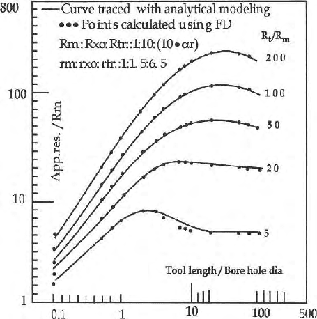
Fig. 15.11. Comparison of analytical and ﬁnite diﬀerence modelling results

nonzero values. The remaining entries are all zeros. Direct solution of the

matrix equation can be done using one of the matrix solvers. For a thick bed,

Fig. 15.11 shows the apparent resistivity curves in the presence of ﬂushed zone,

invaded zone and uncontaminated zone. Finite diﬀerence curves are compared

with those available in Schlumberger Well Surveying Corporation Document

(1972).

15.4 Finite Diﬀerence Formulation Plane Wave

Electromagnetics Magneto t ell urics

In the last two Sects. 15.2 and 15.3, ﬁnite diﬀerence formulations both for

surface a nd borehole geophysics are demonstrated for direct current ﬂow ﬁeld

domain in considerable details where the guiding e q uations were Poisson’s

equation.

In this section we have given a brief structure of the ﬁnite diﬀerence for-

mulations for plane wave electromagnetics using Maxwell’s equations and

Helmholtz electromagnetic wave equations as guiding equations. Boundary

conditions are considerably diﬀerent in electromagnetics. Details of electro-

magnetic boundary conditions are discussed in the Chap. 12.

In Magnetotellurics (MT) two sets of ﬁeld data in frequency domain are

obtained after continuous time domain recording o f electric and magnetic

15.4 Plane Wave Electromagnetics Magnetotellurics 491

ﬁelds in two mutually perpendicular north-south and east-west directions.

Theratiooftheelectricﬁeldtothetransverse magnetic ﬁeld in frequency

domain are obtained after pro cessing and fourier transforming two sets of

time domain E and H ﬁelds. One gets impedances, viz, Z

(= E

)

and Z

). Madden and Nelson (1960) proposed that magnetotelluric

impedance Z is actually a 2 × 2MTtensorwhereZ

and Z

are oﬀ

diagonal elements and Z

and Z

are diagonal elements. In 1967 Swift

brought the concepts of mathematical rotation of the MT impedance ten-

sor, optimum rotation angle and TE(Transverse Electric) and TM(Transverse

Magnetic) mode in 2 -D MT. Swift rotation (1967) equation is given by,

Vozoﬀ(1972),

′

=MZM

(15.48)

where,

′

)

′

. (15.49)

The primed components denote the components of the impedance tensor Z

after rotation. Here

)

cos θ sin θ

−sin θ cos θ

and (15.50)

is the transpose of M .

For a two dimensional (2-D) structures (see Chap. 2) as well as for opti-

mum rotation angle θ, the angle between the geographic north and the strike

direction of the 2-D structure, one gets Z

=0and



′



maximum. The rotated apparent resistivity and phases are given by

′

axy

=0.2T



′



and ϕ

′

=tan

−1





′





′





(15.51)

′

ayx

=0.2T



′



and ϕ

′

=tan

−1





′





′





. (15.52)

Here the rotated primed parameters are the E and H polarization parameters.

They are ρ

, φ

and ρ

, φ

At optimum rotation angle, Helmholtz wave equation ∇



= γ



decouples into two separate independent sets of equations. TE or E

stands

for transverse electric or E-p olarization mode where electric ﬁeld is paral-

lel to the geological strike. TM or E

⊥

stands for transverse magnetic or

H-polarization mode (Table 15.1). Here magnetic ﬁeld is parallel to the

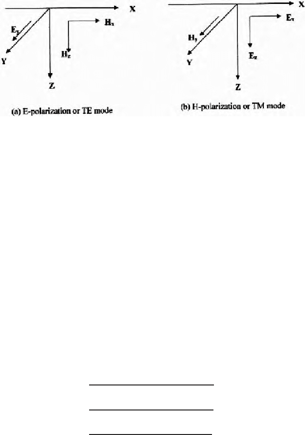
strike and electric ﬁeld is perp endicular to the strike Figs. (15.12) and

(15.13 a, b) respectively show the strike direction in an ideal 2D mo d el

492 15 Numerical Methods in Potential Theory

Table 15.1. Break up of Helmholtz electromagnetic wave equation for E and H

polarisations

E-polarization equations H-polarization equations

i) E = E(0, E

, 0), H = H(H

, 0, Hz)

∂H

∂z

−

∂H

∂x

= σE

−

∂E

∂z

=iωµH

∂E

∂x

=iωµH

−

iωµ

∂

∂z

−

iωµ

∂

∂x

= σE

∂

∂x

∂

∂z

= γ

= −

iωµ

∂E

∂z

iωµ

∂E

∂x

i) E = E(E

, 0, Ez), H = H(0, H

, 0)

−

∂H

∂z

= σE

∂H

∂x

= σE

∂E

∂z

−

∂E

∂x

=iωµH

−

∂

∂z

−

∂

∂x

=iωµσH

∂

∂z

∂

∂x

= γ

= −

∂H

∂z

∂H

∂x

and the directions of electric and magnetic vectors in E-polarisation and H-

polarisation.

Since the low frequencies are involved in MT exploration, conduction cur-

rents dominate over displacement currents. The integral forms of Maxwell’s

equations in mks units can be written as



H.dl =



J.dS =



σE .dS (15.53)



E.dl =



iμωH .dS, (15.54)

where in general, σ and μ are scalars for a homogeneous and isotropic medium

and tensors for inhomogenous and anisotropic medium (Chap. 2). These

Maxwell’s equations and Helmholtz wave equations given in Chaps. 12 and 13

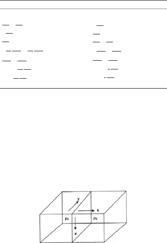
Fig. 15.12. A model of a two dimensional earth with a strike along the y direction;

and ρ

are the resistivities of the two blocks

15.4 Plane Wave Electromagnetics Magnetotellurics 493

Fig. 15.13. Directions of electric and magnetic ﬁelds for E and H polarizations

and in Table 15.1 are used to generate the ﬁnite diﬀerence modelling struc-

tures. We can deﬁne a diﬀerence scheme such that (15.53) or (15.54) are

exactly satisﬁed. Finite diﬀerence scheme in Magnetotellurics proposed by

Mackie et al (1993) are as follows (Fig. 15.14 a,b)

a) The x, y, z components of (15.53) are

{[H

(i, j +1,k) − H

(i, j, k)] −[H

(i, j, k + l)

−H

(i, j, k)]}L = J

(i, j, k) L

{[H

(i, j, k +1)−H

(i, j, k)] − [H

(i +1,j,k)

−H

(i, j, k)]}L = J

(i, j, k) L

(15.55)

{[H

(i +1,j,k) − H

(i, j, k)] − [H

(i, j +1,k)

−H

(i, j, k)]}L = J

(i, j, k) L

{[E

(i, j, k) − E

(i, j −1,k)] − E

(i, j, k)

−E

(i, j, k −1)}L = iω < μ

(i, j, k) L

(b)

(i, j, k)=

[ρ

(i, j, k)+ρ

(i −1,j,k)]

(i, j, k) ,

(i, j, k)=

[ρ

(i, j, k)+ρ

(i, j − 1,k)]

(i, j, k) , (15.56)

(i, j, k)=

[ρ

(i, j, k)+ρ

(i, j, k − 1)]

(i, j, k) .

(c)

{[E

(i, j, k) − E

(i, j, k −1)] −E

(i, j, k)

−E

(i −1,j,k)}L = iω < μ

(i, j, k) L

{[E

(i, j, k) − E

(i −1,j,k)] − E

(i, j, k)

− E

(i, j − 1,k)}L = iω < μ

(i, j, k) L

(15.57)

494 15 Numerical Methods in Potential Theory

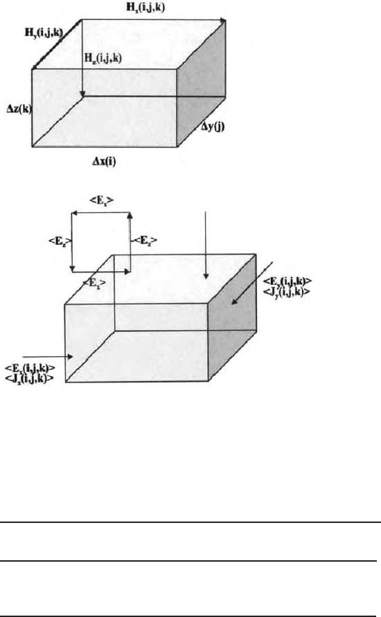
Fig. 15.14. a,b Magnetotelluric ﬁnite diﬀerence rectangular parallelepiped cells

showing the direction of electric and Magnetic Fields (Mackie ,Madden and Wan-

namaker 1993)

where we deﬁne the permeabilities as :

<µ

> =

(i, j − 1,k− 1) + µ

(i, j, k − 1) + µ

(i, j − 1,k)+µ

(i, j, k)

<µ

> =

(i − 1,j,k− 1) + µ

(i, j, k − 1) + µ

(i − 1,j,k)+µ

(i, j, k)

(15.58)

<µ

> =

(i − 1,j− 1,k)+µ

(i − 1,j,k)+µ

(i, j − 1,k)+µ

(i, j, k)

Here ρ and µ the resistivity and magnetic per meability are chosen to be

tensors. E is deﬁned as the average along a co ntour and H is deﬁned as the

average ac ross the surface enclosed by the contours Once the basic equations

for TE and TM mode are available and the guide lines to prepare the diﬀerence

15.4 Plane Wave Electromagnetics Magnetotellurics 495

equations from Maxwell’s equations are obtained one can frame the ﬁnite

diﬀerence formulation program .

15.4.1 Boundary Conditions

In TE mode, the boundary conditions are not simple as E

and H

are all

continuous across the air – earth interface. Consequently, the horizontal H ﬁeld

is not constant everywhere above the ground in the vicinity of a lateral inho-

mogeneity. Thus, it is necessary to consider air layers above the ground . An

upwar d extension of the model cross section upto the air – ionosphere bound-

ary is necessary in an attempt to get numerical solutions for E polarization

problem. This requires an interface, where lateral changes in conductivity do

not exist. Since we need H

=0andE

is constant, a n d ∂E

/∂y = iωμ

ten air layers are generally introduced(Wannamaker 1987). They are the rows

next to the air – earth interface and are of the same height as the rows just

be l ow the surface under the assumption that electric current ﬂow across the

air – earth interface is negligible. These 10 air layers above the surface of the

earthwithexponentialincreased thickness in some cases are chosen such that

the geometric perturbations in the longest wavelength H ﬁeld gets damped.

On top of the air layer an arbitrary electric ﬁeld E o is assumed. Since all the

ﬁelds at diﬀerent depths get normalised, the arbitrary choice is permissible.

The lower half space below the air earth boundary are chosen in such a way

such that Eo = 0 at the bottom. Generally Eo is chosen as 1 above the air lay-

ers. For TM mode modelling air layers are not necessary. Ho also is assumed to

be 1(Ho = 1). The boundary values on the side faces of the model are chosen

from the values obtained from 1D on the surface of the earth. At the bottom of

the half space Ho also is assumed to be zero. Once the boundary conditions are

imposed one gets a series of equations which can be clubbed together to get a

matrix

Ax = b, (15.59)

where b contains terms associated with the known boundary values and source

ﬁeld. This system of equations is sparse, symmetr ic and complex (a l l ele-

ments are real except for the diagonal elements). Once this system has been

solved for the H ﬁelds, the E ﬁelds can be determined by application of curl

H =J=σE neglecting the displacement c u rrent as mentioned. The values of

the electric and magnetic ﬁeld on all the nodes in the model are obtained.It

is interesting to note that the column vector in this case has mostly nonzero

elements.The matrix A is symmetric in this case. In the DC domain, the

matrix A is asymmetric These considerable diﬀerence in boundary condi-

tions and formulation do exist between direct current and electromagnetic

ﬁeld domain. Choice of matrix solver may be diﬀerent. Otherwise step by

step structure of the FD formulation in both the cases are more or less the

same.

496 15 Numerical Methods in Potential Theory

15.5 Finite Element Formulation Direct Current

Resistivity Domain

15.5.1 Introduction

The basic concept in the ﬁnite element method is that a continuous space

domain, is assumed to be composed of a set of piecewise continuous functions

deﬁned over a ﬁnite number of subdomains or elements. The piecewise con-

tinuous space called elements and any function say potential or ﬁeld or stress

or strain are deﬁned using values of continuou s quantity at a ﬁnite number

of point in the sol u ti on domai n assuming linear or nonlinear variations in

polynomials. Discretization of the space domain, elements, nodes, bo u n dary

conditions, use of matrix solver are more or less same as those we discussed in

Sect. 15.2 a nd 15.3. But the solution of the problem in ﬁnite element (FEM)

domain is considerably diﬀerent from what we have seen in Sect. 15.2 and 15.3.

The steps involved in formulating a problem in the ﬁnite element domain may

be summarised as follows:

1) The solution domain is made ﬁnite and divided into a ﬁnite number of

elements, each having suitable physical property assigned. These elements may

be one, two, or three-dimensional according to the problem being considered.

The shape of the elements can be one of the many diﬀerent forms (Zienkiewicz,

1971) viz., triangle, quadrilateral, rectangle, square, tetrahedron, cube, paral-

lelepiped etc with straight or curved boundaries. 2) The elements are intercon-

nected at common nodal points situated at the element boundaries or vertices.

A parameter for the unknown potentials to be determined is assigned to each

of these elements, and the potentials will be obtained from these nodal points.

3) A polynomial function is chosen to deﬁne the behaviour of potential ﬁeld

within the element, in terms of the nodal values. The interpolating polyno-

mial may b e linear, quadratic, or cubic. 4) The approximating p olynomial

functions are then substituted for the true solution into the equation describ-

ing the potential or ﬁeld behaviour. 5) The summation of all the elemental

equations gives an approximation to the equation for the continious potential

function. A system of equations is obtained from which the nodal potentials

may be obtained. 6) One of the approaches viz, Rayleigh Ritz energy mini-

mization method based on variational calculus or the Galerkin’s weights are

chosen. 7) Natural coordinates with isoparametric elements are also used to

bring in curved boundaries. In the p resent ﬁnite element approximation, the

cross-section of a 2-D structur e is represented by a number of triangular ele-

ments. Inside each of these elements a linear behaviour of potential ﬁeld is

assumed. The nodes of the elements are situated at the vertices of the triangles

to which these variables are assigned. The approximation of a two dimensional

ﬁeld variable φ, within an element, e, may be written in terms of the element

unknown parameters φ

as,





(15.60)

15.5 Finite Element Formulation Direct Current Resistivity Domain 497

where β =i, j, k,.........r, r is the number of unknown parameters and

, β =i, r are the element shape functions.

The element shape functions cannot be chosen arbitrarily because these

functions have to satisfy the continuity and convergence requirements of the

method. More details concerning the types of element shape functions ar e

given in Kardestuncer (1987).

One can derive the ﬁnite element form of the governing diﬀerential equa-

tion of a problem in diﬀerent ways. In the present ﬁnite element analysis the

variation al approach is used where a functional is minimised. In the next sec-

tions, GalerKin’s method of ﬁnite element analysis without and with use of

the isoparametric elements are demonstrated.

In this Rayleigh-Ritz approach, a physical problem, governed by a diﬀer-

ential equation, may be equivalently expressed as an extremum problem by

the method of calculus of variations. For the steady state ﬁeld problems, the

ﬁeld equation to be solved is the quasi harmonic equation expressed in general

terms as

∂

∂x



∂φ

∂x



∂

∂y



∂φ

∂y



∂

∂z



∂φ

∂z



= −∇.J

(15.61)

It is shown, by means of the calculus of variations, that a physical problem

deﬁned by the above diﬀerential equation is identical to that of ﬁnding a

function φ, that minimizes a functional ψ. The same boundary conditions

applied to the diﬀerential equation are applicable to this integral equation

ψ =



)



∂φ

∂x



+ σ



∂φ

∂y



+ σ



∂φ

∂z



− 2φ∇.J

dν. (15.62)

Minimization of this functional with respect to the unknown function φ,gives

the potential φ, which also satisﬁes the diﬀerential equation (Coggon 1971).

In this resistivity problem, this integral is associated with power dissipation

within the conducting medium. The minimum condition thus requires that

the potential distribution within the medium is such that the power dissi-

pated (Joule heat in this case) is minimum Reddy (1986). A brief derivation

of the power integral expressed in terms of potential and suitable for direct

applications of the ﬁnite element method is given. Inverse fourier cosine trans-

form discussed in Sect. 15.2 regarding transformation of line source p otential

to point source potential is applicable here also

15.5.2 Derivation of the Functional from Power Considerations

Coggon (1971), Mwinifumb o (1980), Reddy (1986), Silvester and Haslam

(1972), Zienkiewicz and Taylor (1987) have presented the mathematical treat-

ments of the approaches based on the variational calculus. This mathematical

treatment is given by Mwinifumbo (1980) The power dissipated per volume

in a conducting medium with resistivity, ρ and current density, J

,is

498 15 Numerical Methods in Potential Theory

= ρJ

. (15.63)

The relations J

= σE, and E = −∇φ allow the equation to be written as

= σ(∇φ)

(15.64)

If there is a current source within the volume, the power dissipated per unit

volume by the source is

= −J

.∇φ. (15.65)

The power supplied by the source to the ﬁeld is equal to the total power

dissipated as Joule heat, that is,

σ(∇φ)

.∇φ =0. (15.66)

We wish to minimize the power dissipated within a volume where there

is a source, but the function describing the dissipated power and the power

supplied by the source is zero. This problem is handled by a method similar

to the Lagrangian multiplier method. Instead of minimizing the Joule heat

directly (which does not have the source terms), we construct a new function

as follows

σ(∇φ)

.∇φ = 0 (15.67)

which in essence is just the negative of the power supplied to the unit volume.

The integral form of power dissipation within the solution domain is then

given as

ψ =





σ (∇φ)

+2J

.∇φ



dν. (15.68)

Using the identity

∇.(φJ

)=J

.∇φ + φ∇.J

(15.69)

the ﬁrst term on the right hand side of (15.69) may b e written as



.∇φ)dν =



[∇. (φJ

) −φ∇.J

]dν. (15.70)

Applying the divergence theorem to the ﬁrst term on the right hand side of

this equation, we have



.∇φ)dν =



φJ

.nds −



φ∇.J

dν (15.71)

since there are no sources on the surface of the solution domain, the surface

integral vanishes, then



.∇φ)dν = −



φ∇.J

dν. (15.72)