Roy K.K. Potential theory in applied geophysics
Подождите немного. Документ загружается.


15.5 Finite Element Formulation Direct Current Resistivity Domain 499
Equation (15.69) then becomes:
ψ =
ν
σ (∇φ)
2
− 2φ∇.J
s
dν. (15.73)
The current density in a conducting medium is distributed in such a way that
the power dissipated (ohmic power) is minimum. This minimization principle
may be written as
∆ψ =∆
ν
σ (∇φ)
2
− 2φ∇.J
s
dν = 0 (15.74)
where ∆ψ is the variation of the total power ψ with change of the function φ
(x, y, z). This equation is known as the variational equation. In the present
study we will be modeling two-dimensional structures in the presence of 3-D
sources. If we apply a Fourier cosine transform along the Y direction (strike
direction of the 2-D structure being considered), then the variational equation
reduces to
∆ψ =
A
∆
σ
φ
2
x
+ λ
2
φ
2
+ φ
2
z
− 2φIδ (x) δ (z)
dA = 0. (15.75)
Integration is now over ar ea instead of a volume. By using the variational
method, it is shown below that the variation of the power leads to Pois-
son’s differential equation. This is the basis for most methods of calculating
potential distributions and is known as Ray leigh - Ritz energy minimisation
method.
15.5.3 Equivalence between Poisson’s Equation
and the Minimization of Power
Integration and taking the variation in the above equation may be inter-
changed as follows,
∆ψ =
A
∆
σ
φ
2
x
+ λ
2
φ
2
+ φ
2
z
− 2φIδ (x) δ (z)
dA = 0. (15.76)
Differentiation and the operation of variation may also b e interchanged, thus
enabling the (15.76) to be written a s
∆ψ =
A
σ
φ
x
.
∂ (∆φ)
∂x
+ λ
2
φ (∆φ)+φ
z
.
∂ (∆φ)
∂z
− I(∆φ) δ (x) δ (z)
dA = 0.
(15.77)
Integrating the first term under the integral in (15.77) in the square brackets
yields
500 15 Numerical Methods in Potential Theory
A
∂φ
∂x
.
∂∆φ
∂x
dA =
A
∂
∂x
∂φ
∂x
.∆φ
dA −
A
∂
∂x
∂φ
∂x
∆φ
dA. (15.78)
Applying the divergence theorem to the first integral on the right hand side
of (15.78), we get
A
∂φ
∂x
∂ (∆φ)
∂x
dA =
L
l
x
∂φ
∂x
∆φ
dL −
A
∂
∂x
∂φ
∂x
∆φ
dA (15.79)
where l
x
is the direction cosine of the normal to the exterior boundary with
respect to the X-axis, and L is the bounding contour of the solution domain
area. A performing similar operations on the third term of the square brackets
of (15.77) gives
A
∂φ
∂z
∂ (∆φ)
∂z
dA =
L
l
z
∂φ
∂z
∆φdL −
A
∂
∂z
∂φ
∂z
∆φ
dA. (15.80)
On substitution of the expression (15.79) and (15.80) into the variational
equation we get
∆ψ =
A
σ
∂
2
φ
∂x
2
+ λ
2
φ +
∂
2
φ
∂x
2
− Iδ (x) δ (z)
(∆φ)dA
+
L
σ
l
x
∂φ
∂x
+l
z
+
∂φ
∂z
(∆φ) dL = 0 (15.81)
When the boundary values are given, ∆φ = 0 on L, the line integral vanishes.
When the boundary values are not given, the variation of φ on L is in general
nonzero. Since the variation of φ within the solution domain is not necessarily
zero, ∆ψ = 0 occurs only if the square bracketed terms within the integral
vanishes. This requirement yields the following equations.
σ
∂
2
φ
∂x
2
− λ
2
φ +
∂
2
φ
∂z
2
+Iδ (x) δ (z)] = 0
σ
l
x
∂φ
∂x
+l
z
∂φ
∂z
= 0 (15.82)
The first part o f (15.82) is Poisson’s equation with a Fourier cosine trans-
formation applied along the Y direction and the second part is the natural
boundary condition (homogeneous Neumann boundary condition).
15.5.4 Finite Element Formulation
This formulation is based on the work of Mwinifumbo (1980), Zienkiewicz
and Taylor (1989), Reddy (1986), Krishnamurthy (1991) Roy and Jaiswal
15.5 Finite Element Formulation Direct Current Resistivity Domain 501
(2001) (Fig. 15.5). In the present analysis a linear polynomial and triangular
elements are used, that is, the function φ is taken to vary linearly over the
triangular element with nodes at the vertices (Fig. 15.15).
Let a given triangular element with nodes i, j, k and coordinates of the
three nodes being (x
i
,z
I
), (x
j
,z
j
)and(x
k
,z
k
), have the following nodal values
of the potential function φ; φ
i
, φ
j
, φ
k
.
The interpolating polynomial is
φ = α
1
+ α
2
x+α
3
z (15.83)
with the nodal conditions
φ = φ
I
at x = x
i
, z=z
i
(15.84)
φ = φ
j
at x = x
j
, z=z
j
φ = φ
k
at x = x
k
, z=z
k
.
Substituting of these nodal values into (15.83), one gets a system of equations.
φ
i
= α
1
+ α
2
x
i
+ α
3
z
i
φ
j
= α
1
+ α
2
x
j
+ α
3
z
j
(15.85)
φ
k
= α
1
+ α
2
x
k
+ α
3
z
k
which yield
Fig. 15.15. A triangular finite element showing the coordinates of the nodes

502 15 Numerical Methods in Potential Theory
α
1
=
1
2A
'
(x
j
z
k
− x
k
z
j
) φ
i
+(x
k
z
i
− x
i
z
k
) φ
j
+(x
i
z
j
− x
j
z
i
) φ
k
(
α
2
=
1
2A
'
(z
j
− z
k
) φ
i
+(z
k
− z
i
) φ
j
+(z
i
− z
j
) φ
k
(
α
3
=
1
2A
'
(x
k
− x
j
) φ
i
+(x
j
− x
k
) φ
j
+(x
j
− x
i
) φ
k
(
(15.86)
where 2A is equa l to
2A =
1x
i
z
i
1x
j
z
j
1x
k
z
k
(15.87)
A being the area of the triangle.
When the value of α
1
, α
2
and α
3
are substituted into the expression for
the interpolating polynomial, the following element equation is obtained after
the terms have been rearranged i.e.,
φ
e
=N
i
φ
i
+N
j
φ
j
+N
k
φ
k
(15.88)
where φ
e
is the potential over the element, e, and N
i
,N
j
and N
k
are the three
shape functions associated with each node of the triangular element and are
defined as follows:
N
i
=
1
2A
(a
i
+ b
i
x + c
i
z)
N
j
=
1
2A
(a
j
+ b
j
x + c
j
z) (15.89)
and
N
k
=
1
2A
(a
k
+ b
k
x + c
k
z)
where,
a
i
=x
j
z
k
− x
k
z
j
b
i
=z
j
− z
k
(15.90)
c
i
=x
k
− x
j
a
j
=x
k
z
i
− x
j
z
k
b
j
=z
k
− z
i
(15.91)
c
j
=x
i
− x
k
and
a
k
=x
i
z
j
− x
j
z
i
b
k
=z
i
− z
j
(15.92)
c
k
=x
j
− x
i
.
15.5 Finite Element Formulation Direct Current Resistivity Domain 503
The potential function φ is thus a function of a set of shape functions which
are linear in x and z. This means that the gradients in either x or z direction
will be constant. These are determined as follows:
∂φ
e
∂x
=
∂N
i
∂x
φ
i
+
∂N
j
∂x
φ
j
+
∂N
k
∂x
φ
k
∂φ
e
∂z
=
∂N
i
∂z
φ
i
+
∂N
j
∂z
φ
j
+
∂N
k
∂z
φ
k
(15.93)
The partial derivatives of the shape functions with respect to x and z axes are
evaluated as follows:
∂N
β
∂x
=
1
2A
b
β
∂N
β
∂z
=
1
2A
c
β
(15.94)
β =i, j, k.
Therefore, (15.93) reduce to
∂φ
e
∂x
=
1
2A
b
i
φ
i
+b
j
φ
j
+b
k
φ
k
∂φ
e
∂z
=
1
2A
c
i
φ
i
+c
j
φ
j
+c
k
φ
k
. (15.95)
The parameters b
i
,b
j
,b
k
,c
i
,c
j
,c
k
are constants (they are fixed once the
nodal coordinates are specified) and φ
i
, φ
j
and φ
k
are independent of the
space coordinates. Figure 15.16 shows Dirichlet and Neuman boundaries in a
FEM problem with triangular elements as shown in Sect. 15.2.
15.5.5 Minimisation of the Power
When we minimize the power defined by (15.68), it is only required to derive
that the necessary conditions for a typical element. Influence of other elements
will follow an identical pattern. To obtain the general equation, we simply add
contributions of all the elements.
The power dissipated in an element, e, defined by nodes i, j, and k is given
as (if there are no sources within the element).
ψ
e
=
e
σ
)
∂φ
e
∂x
2
+ λ
2
φ
e2
+
∂φ
e
∂z
2
*
dxdz. (15.96)
On substitution of the nodal values and their derivatives (15.96) becomes
ψ
e
=
e
σ
4A
2
(b
i
φ
i
+ b
j
φ
j
+ b
k
φ
k
)
2
+ λ
2
(N
i
φ
i
+ N
j
φ
j
+ N
k
φ
k
)
+(c
i
φ
i
+ c
j
φ
j
+ c
k
φ
k
)
2
dx dz. (15.97)
504 15 Numerical Methods in Potential Theory
Fig. 15.16. A finite triangular element mesh showing the working and adjoining
areas, Dirichlet and Neumann conditions at the boundaries
To obtain the minimum of the power within an element, the differentials of ψ
e
with respect to the nodal parameters φ
i
, φ
j
, φ
k
are evaluated first. To illustrate
the procedure of obtaining these differentials, (15.96) is differentiated with
respect to the nodal values
φ
.
∂ψ
e
∂φ
i
=
σ
2A
'
b
2
i
+ c
2
i
φ
i
+(b
2
b
j
+ c
2
c
j
) φ
j
+(b
j
b
k
+ c
k
c
i
) φ
k
(
e
dxdz
+2σx
2
e
'
N
2
i
Kφ
i
+ N
i
N
j
K
j
+
(
. (15.98)
The integrals in the above equation are taken over the area of the element.
Integration is straight forward when the triangular area coordinates, L
1
,L
2
,L
3
(Zienkiewicz (1971)) a re used. These coordinates specify the position of any
point within the triangle by giving the distance measured perpendicularly
from each side to the point, distances being expressed as fractions of the
triangle altitude.
The area co ordinates span the range of numerical values from 0 to 1 in
any triangle. For a triangular element with corners numbered 1, 2 and 3, these
area coordinates are related to the x and z coordinates by
⎡
⎢
⎣
L
1
L
2
L
3
⎤
⎥
⎦
=
1
2A
⎡
⎢
⎣
(x
2
z
3
− x
3
z
2
)(z
2
− z
3
)(x
3
− x
2
)
(x
3
z
1
− x
1
z
3
)(z
3
− z
1
)(x
1
− x
3
)
(x
1
z
2
− x
2
z
1
)(z
1
− z
2
)(x
2
− x
1
)
⎤
⎥
⎦
⎡
⎢
⎣
1
x
z
⎤
⎥
⎦
. (15.99)
15.5 Finite Element Formulation Direct Current Resistivity Domain 505
Using these coordinate variables, which are also the shape functions for the
linear element; that is
N
i
=L
1
N
j
=L
2
N
k
=L
3
We have
A
L
a
1
L
b
2
L
c
3
dA =
a!b!c!
(a+b+c+2)!
2A (15.100)
where a, b, c are the p owers of the coo rdinates Using the above equation the
integrals in (15.98) are evaluated as
e
dxdz = A
e
'
N
2
i
φ
i
+ N
i
N
j
φ
j
+ N
i
N
k
φ
k
(
dxdz =
A
6
φ
i
+
A
12
φ
j
+
A
12
φ
R
. (15.101)
Equation (15.98) reduces to
∂ψ
e
∂φ
i
=
σ
2A
(b
i
+ t
i
jφ
j
+ t
i
kφ
k
)+
λ
2
σA
6
(2φ
i
+ φ
j
+ φ
k
) (15.102)
where
t
ii
=(z
j
− z
k
)
2
+(x
k
− x
j
)
2
t
ij
=(z
j
− z
k
)(z
k
− z
j
)+(x
k
− x
i
)(x
i
− x
k
) (15.103)
t
ik
=(z
j
− z
k
)(z
i
− z
j
)+(x
k
− x
i
)(x
j
− x
i
).
For the whole element i, j, k the differentiation of the power integral is with
respect to the parameters φ
i
, φ
j
, φ
k
. In matrix notation, the elemental system
of equations may be written as
∂ψ
∂φ
e
=
⎡
⎢
⎢
⎢
⎣
∂ψ
e
∂φ
i
∂ψ
e
∂φ
j
∂ψ
e
∂φ
k
⎤
⎥
⎥
⎥
⎦
. (15.104)
The coefficients of φ
′
s for each element form two symmetric (3 × 3) element
matrices
σ
2A
⎡
⎣
b
2
i
+ c
2
i
(b
i
b
j
+ c
i
c
j
)(b
i
b
k
+ c
i
c
k
)
(b
i
b
j
+ c
i
c
j
)
b
2
j
+ c
2
j
(b
j
b
k
+ c
j
c
k
)
(b
i
b
k
+ c
i
c
k
)(b
j
b
k
+ c
j
c
k
)
b
2
k
+ c
2
k
⎤
⎦
and
λ
2
σA
6
⎡
⎣
211
121
112
⎤
⎦
. (15.105)
506 15 Numerical Methods in Potential Theory
The final equations for minimising total power within the solution domain are
assembled by adding the contributions of each element to a typical differential
and equating the result to zero. Thus
∂ψ
∂φ
i
=
N
β=1
∂ψ
β
∂φ
i
= 0 (15.106)
where N is the number of elements sharing the node i. It should be noted
that for a particular node i only the values of φ at nodes connected to it
will appear and that the coefficients will involve only contributions from the
elements adjacent to the node being considered. This results into a typical
narrow band ed coefficient matrix for a set of simultaneous equations. If the
potential function φ is to be determined at M number of nodes, then a set of
M linear simultaneous equations result. The required values φ
1
, φ
2
.....φ
M
are
obtained u pon solving these equations. In matrix form, the equations may be
written as
[T] {φ} = {S} (15.107)
where [T] is the matrix of coefficients of the equation, φ is the column vec-
tor of M unknown potential values and S is the column vector containing
source terms extracted from the right-hand side of (15.107). The matrix [T] is
a large, symmetric, diagonally dominant, penta diagonal and sparse matrix.
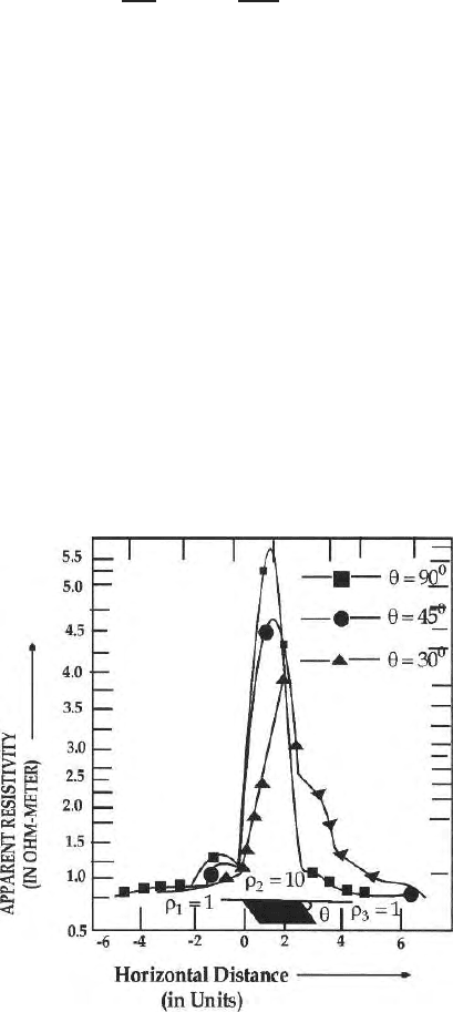
Fig. 15.17. Two electrode profile over a dipping dyke
15.6 3D Model 507
That is, most of the terms in any one row are zeros and the non-zero terms
are restricted to a band about the diagonal. Only non-zero terms need to be
stored in along with a ppropriate locations in the matrix. That reduces con-
siderable amount of storage space needed on the computer. Since the matrix
is symmetrical about the diagonal, only one half of the non-zero terms need
to be stored . Integral transform to change the line source respo nse to point
source response, implementation of Dirichlet and Neumann boundary condi-
tions and generation of expanding grids a re more or less the same as discussed
in Sect. 15.2. Figure (15.17) show the theoretically computed two electrode
profiles acro ss a dipping dyke using FEM source code.
15.6 3D Model
Three Dimensional space is divided into discrete tetrahedral elements. The
space consists of a working volume with small tetrahedrons and the outer
volume with large and exponentially expanding elements intended for appli-
cation of the Dirichlet’s boundary conditions. The process of division is two
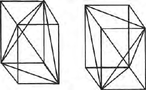
fold. The whole volume is first divided into octahedral elements. These octa-
hedral elements are divided into five tetrahedrons each. The division of these
octahedral elements leads to two different arrangements of the tetrahedrons
(Fig. 15.18a,b). In order to generate the stiffness matrix, a suitable polynomial
approximation is chosen to fit the potential variation within the tetrahedral
elements. Standard linear polynomial is given by
ϕ = α
1
+ α
2
x+α
3
y+α
4
z (15.108)
where α
1
, α
2
, α
3
, α
4
are constants. On this basis we prepare the element stiff-
ness and hence the global stiffness matrix as follows: Consider a tetrahe-
dral element having the coordinates (x
I
,y
I
,z
I
), (x
j
,y
j
,z
j
), (x
k
,y
k
,z
k
)and
(x
p
,y
p
,z
p
) with potential values φ
i
,φ
j
,φ
m
and φ
p
at i
th
,j
th
,m
th
and p
th
node
respectively.
The nodal conditions are
Fig. 15.18. Tetrahedral elements for a 3D Finite element problem
508 15 Numerical Methods in Potential Theory
φ = φ
i
at x = x
i
,y = y
i
,z = z
i
φ = φ
j
at x = x
j
,y = y
j
,z = z
j
φ = φ
m
at x = x
m
,y = y
m
,z = z
m
(15.109)
φ = φ
p
at x = x
p
,y = y
p
,z = z
p
.
Writing in matrix form
⎡
⎢
⎢
⎣
φ
i
φ
j
φ
m
φ
p
⎤
⎥
⎥
⎦
=
⎡
⎢
⎢
⎣
1 x
i
y
i
z
i
1 x
j
y
j
z
j
1 x
m
y
m
z
m
1 x
p
y
p
z
p
⎤
⎥
⎥
⎦
×
⎡
⎢
⎢
⎣
α
1
α
2
α
3
α
4
⎤
⎥
⎥
⎦
(15.110)
Or
⎡
⎢
⎢
⎣
α
1
α
2
α
3
α
4
⎤
⎥
⎥
⎦
=
⎡
⎢
⎢
⎣
a
11
a
12
a
13
a
14
a
21
a
22
a
23
a
24
a
31
a
32
a
33
a
34
a
41
a
42
a
43
a
44
⎤
⎥
⎥
⎦
×
⎡
⎢
⎢
⎣
φ
i
φ
j
φ
m
φ
p
⎤
⎥
⎥
⎦
. (15.111)
The power dissipation in an element (with no sources within) is given by
ψ
e
=
v
o[(
∂φ
e
∂x
)+(
∂φ
e
∂y
)
2
+(
∂φ
e
∂z
)
2
]dv. (15.112)
To obtain minimum power within an element, the derivatives of ψ
e
with
respect to φ
i
,φ
j
,φ
m
and φ
p
are equated to zero.
∂ψ
∂φ
e
=
⎡
⎢
⎢
⎢
⎢
⎢
⎢
⎢
⎣
∂ψ
e
∂φ
i
∂ψ
e
∂φ
i
∂ψ
e
∂φ
m
∂ψ
e
∂φ
p
⎤
⎥
⎥
⎥
⎥
⎥
⎥
⎥
⎦
. (15.113)
Alternatively the element stiffness matrix is
∂ψ
∂φ
e
= V ×
⎡
⎢
⎢
⎣
a
21
a
21
+ a
31
a
31
+ a
41
a
41
a
21
a
22
+ a
31
a
32
+ a
41
a
42
a
21
a
22
+ a
31
a
32
+ a
41
a
42
a
22
a
22
+ a
32
a
32
+ a
42
a
42
a
21
a
23
+ a
31
a
33
+ a
41
a
43
a
22
a
23
+ a
32
a
33
+ a
42
a
43
a
21
a
24
+ a
31
a
34
+ a
41
a
44
a
22
a
24
+ a
32
a
34
+ a
42
a
44
a
21
a
23
+ a
31
a
33
+ a
41
a
43
a
21
a
24
+ a
31
a
34
+ a
41
a
44
a
22
a
23
+ a
32
a
33
+ a
42
a
43
a
22
a
24
+ a
32
a
34
+ a
42
a
44
a
23
a
23
+ a
33
a
33
+ a
43
a
43
a
23
a
24
+ a
33
a
34
+ a
43
a
44
a
23
a
24
+ a
33
a
34
+ a
43
a
44
a
24
a
24
+ a
34
a
34
+ a
44
a
44
⎤
⎥
⎥
⎦
(15.114)
The element stiffness matrix is mapped into the global stiffness matrix element
by element. Assembly of all the equations gives