Ockendon J., Howison S., Lacey A., Movchan A. Applied Partial Differential Equations
Подождите немного. Документ загружается.

68
FIRST-ORDER QUASILINEAR SYSTEMS
u=v=0 ony=O
have no analytic solution in a neighbourhood of y = 0 unless f is real and analytic.
To see this, note that u - f + iv is an analytic function whose real part is -f on
y = 0 and whose imaginary part is zero on y = 0.
This is already a striking result, but it only ensures non-existence of solutions
of (2.61) locally near y = 0. However, it is the starting point for H. Lewy's famous
demonstration that, even though f (x, y, t) may be CIO at every point in R3, the
linear partial differential equation
8u
i
8u
- 2i(x+iy)
8u
= f (x, y, t)
8x+ay
St
has no solution at all unless f is in addition analytic. The details are too lengthy
to reproduce here and we refer any reader who wishes to see the futility of trying
to construct an all-embracing theory of partial differential equations to (23, 36].
Exercises
2.1. Show that, if ry = 2 and p/p2 is constant, the gasdynamic equations (2.3) and
(2.4) reduce to the shallow water equations (2.1) and (2.2), with p in (2.3)
and (2.4) proportional to h in (2.1) and (2.2).
2.2. Show that when the substitution proposed before (2.8) is made in (2.5)-(2.7)
and squares of barred quantities are neglected, we obtain
T. (Pou+UP)+
y(pov)=0,
On
=-poe,
Ue =-port.
Show also that
p PO
P P
(1+ \1
-ryPo/)
in this approximation and hence deduce (2.8)--(2.10).
2.3. In a granular material, let the forces on the sides of a rectangle of area baby
be (a, r) by on a side normal to the x axis and (r, ay) bx on a side normal
to the y axis, as in Fig. 2.20. Show that the forces on the diagonal are
cbs = (ayby+Tbx,a.bx+Tby)
and hence that
Now define
or = (ascos0+Tsin0,a.sin0+rcos0).
a2 +a
Vtan 20 =
27
P=-
2
as -
ay.
Show that the components of a along and perpendicular to n are
_
cos 2(t1 - 0) sin 2(r0 r - 0)
o"
-P +
T
sin 20
EXERCISES 69
(r, ay) 8x
(17X , T) By
Fig. 2.20 Forces on an element of a granular medium.
Fig. 2.21 The Mohr circle.
respectively. Deduce that
(a + p)2 + rr = r2 cosec2 20,
a relation which is known as the Mohr circle in the (a,,, re) plane (see
Fig. 2.21).
Identify the region in this figure that corresponds to the fric-
tion constraint Ire/anI 5 tan 0, show that in limiting equilibrium
r = psin0sin20, o- f = -p(1 - sin0cos2ji),
a, = -p(1 +sin0cos20),
and hence deduce (2.16) when p > 0.
2.4.
(i) The discussion on p.46 is equivalent to writing
820 02
8x2 + 8y2 -
0
as a first-order system of dimension 2 by setting
00
00
-u.
8x
TO FIRST-ORDER QUASILINEAR SYSTEMS
Can
z z
axe+42+0=0
be written as a system of dimension 2?
(ii) Show that, if A and B are constant matrices and
u=
then
u2
Cul)
8
+
=0
can be written as a scalar second-order equation for ul or u2. Would the
same be true for a system with non-constant coefficients A and B?
2.5. Consider the non-autonomous inhomogeneous Cauchy problem
8u
= D(u, x, y) 5j + d(u, x, y),
8x
u=uo onx=O.
8x=0
with
r1=y onx=O
Ot on
Ox Oy
with
t=0 onx=O,
and setting
0
show that v satisfies the autonomous homogeneous Cauchy problem
with
v=vo onx=O,
where
D 0 d uo
D = OT 0 1
and
vo = 0
OT00 y
EXERCISES 71
2.6.
(i) Show that the solution of
8u
Ou
= uay,
8x
with u(0, y) = y, is u = y/(1- x).
(ii) For this example, in the notation of §2.3, d(u) = u and uo(y) = y. What
are R. and Rd? Take pa = pd = p > 0 and show that M. = Md = P.
Deduce that D(U) = p2/(p - U) and Uo(y) = py/(p - y), and hence
that the solution of OU/Ox = D(U) OU/Oy is given implicitly by
_p2x pU
Y= p-U+ p+U'
Deduce that U blows up on the lower branch of the parabola
y=
2
(1-x±2fx).
The distance from the nearest point on this curve to the origin controls
the radius of convergence of (2.35); how does this distance depend on p?
2.7. Suppose that
A
au
+ B
Ou
= c,
and A is invertible. Suppose also that the row vector IT is such that
IT (01- 2A-' B) = OT,
(2.62)
where (.,y) is such that (x(t),y(t)) is a characteristic. Show that ITU =
ITA-'ci, which is (2.27).
2.8. Suppose that a hyperbolic system can be written in terms of the Riemann
invariants r1,2 as
8x + A1(rl , r2)
8y)
rl =
0,
(8x + A2 (rl,
r2)
p.. J
r2 = 0.
Show that x and y satisfy the linear system V N /
8r2
= Al(rl,r2)ur2,
2.9. Write the system
in the form
8y
Ox
ey
ex
5,1 = A2(rl,r2)iirl .
Ou Ou Ov
F+-0'
8
+ey+2 + =0,
Ox-ay+2ay=0,
8x
+B-
Oy
=0
,
and show that it is hyperbolic with dy/dx = A = ±1, 3 on the characteristics.
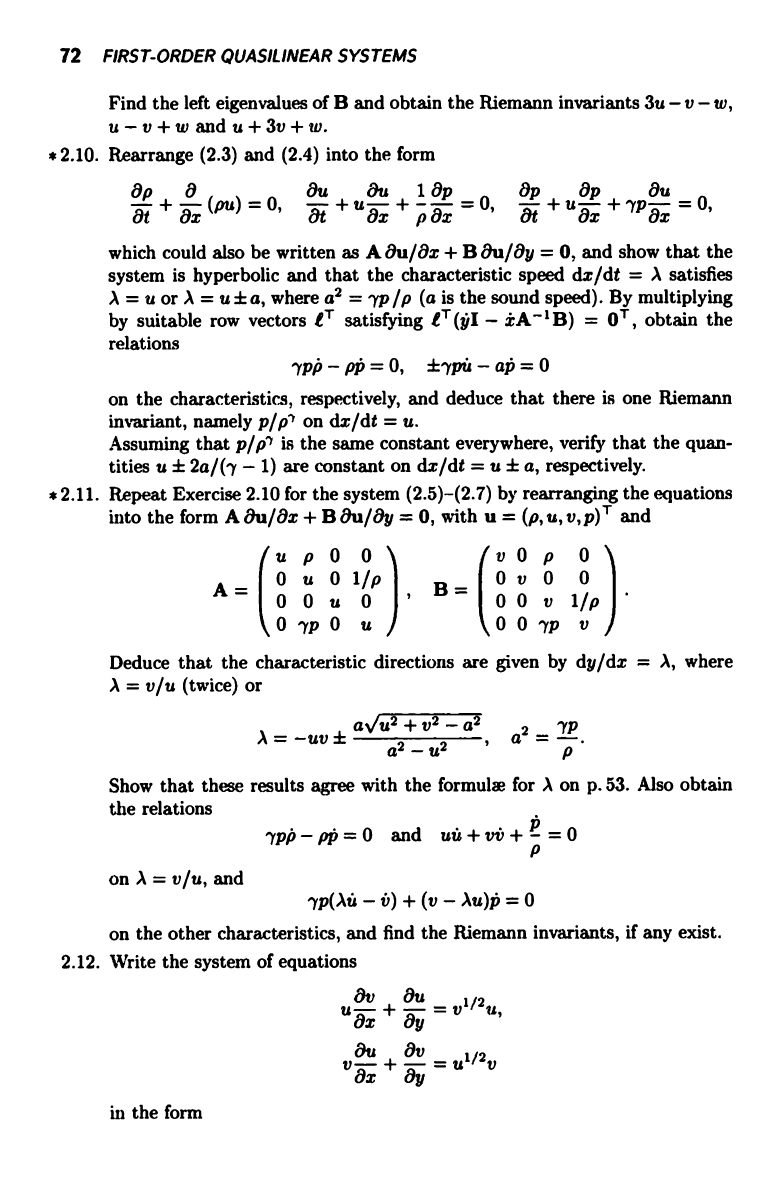
72
FIRST-ORDER QUASILINEAR SYSTEMS
Find the left eigenvalues of B and obtain the Riemann invariants 3u - v - w,
u-v+w and u+3v+w.
* 2.10. Rearrange (2.3) and (2.4) into the form
op
0 On
au
lap ap
ap
On
+-(pu) =0,
+u-+-- =0, +u-+yp- =0,
at ax
at ax p ax
at
ax ax
which could also be written as AOu/ax + B au/ay = 0, and show that the
system is hyperbolic and that the characteristic speed dx/dt = A satisfies
A = u or A = u±a, where a2 = 7P /p (a is the sound speed). By multiplying
by suitable row vectors tT satisfying tT (yI - iA-'B) = OT, obtain the
relations
7pp-pP=0, ±ypri-ap=0
on the characteristics, respectively, and deduce that there is one Riemann
invariant, namely p/p"' on dx/dt = u.
Assuming that p/p'' is the same constant everywhere, verify that the quan-
tities u ± 2a/(-t - 1) are constant on dx/dt = u ± a, respectively.
s 2.11. Repeat Exercise 2.10 for the system (2.5)-(2.7) by rearranging the equations
into the form A au/ax + B au/ay = 0, with u = (p, u, v, p) T and
u p 0 0
v 0 p 0
_
O u 0 1/p
0 v 0 0
0 0 u 0
B_
- 0 0 v
1/p
O yp0 u
OOyp V
Deduce that the characteristic directions are given by dy/dz = A, where
A = v/u (twice) or
-UV ±
a u +v -a
,
a2=LP.
A=
a2-u2
P
Show that these results agree with the formulae for A on p.53. Also obtain
the relations
7PP-pP=0
and uu+vv+p =0
p
on A = v/u, and
yp(Au-v)+(v-Au)p=0
on the other characteristics, and find the Riemann invariants, if any exist.
2.12. Write the system of equations
av
On
u-
+ =
y
v-
+
=u
1/2
V
v
in the form
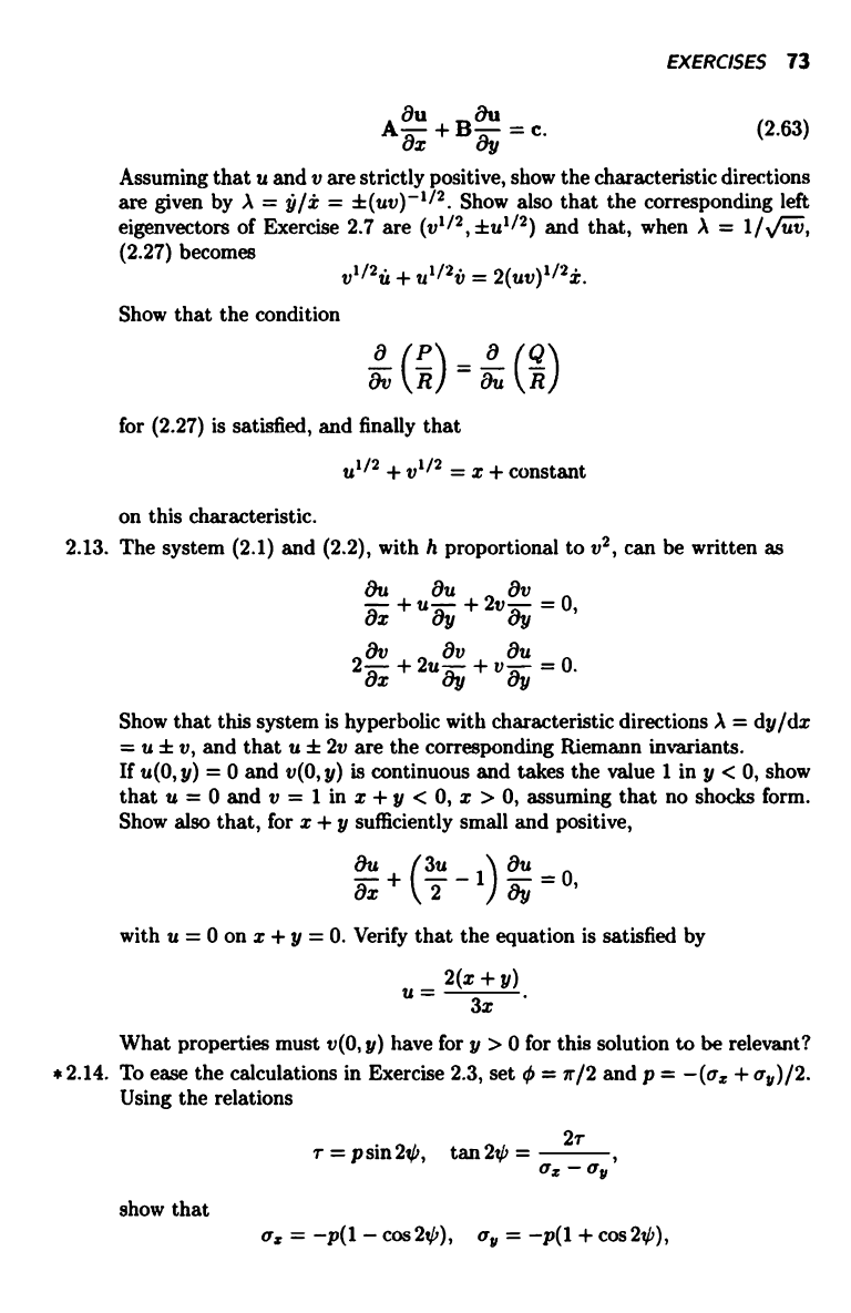
EXERCISES 73
A
TX
+ B ji = c.
(2.63)
Assuming that u and v are strictly positive, show the characteristic directions
are given by A = y/i = ±(uv)-112. Show also that the corresponding left
eigenvectors of Exercise 2.7 are (v1/2,±u1/2) and that, when \ = 1/ uv,
(2.27) becomes
Show that the condition
v1/2ie + u1/2iu = 2(uv) 1/2i.
8;
(R) 8u (R)
11
for (2.27) is satisfied, and finally that
u1/2 + v1/2 = x + constant
on this characteristic.
2.13. The system (2.1) and (2.2), with h proportional to v2, can be written as
a
+uay+2vOy=0,
2Ox + 2u
ey Oy = 0.
Show that this system is hyperbolic with characteristic directions A = dy/dx
= u ± v, and that u ± 2v are the corresponding Riemann invariants.
If u(0, y) = 0 and v(0, y) is continuous and takes the value 1 in y < 0, show
that u = 0 and v = 1 in x + y < 0, x > 0, assuming that no shocks form.
Show also that, for x + y sufficiently small and positive,
8
+(32 -1)O u-0,
\l
JJ
with u = 0 on x + y = 0. Verify that the equation is satisfied by
2(x + y)
U
3x
What properties must v(0, y) have for y > 0 for this solution to be relevant?
+2.14. To ease the calculations in Exercise 2.3, set 0 = it/2 and p = -(a. +oy)/2.
Using the relations
T = p sin 20,
tan 20 =
27-
Qz - oy'
show that
a. = -p(1 - cos 2t'),
ay = -p(1 + cos 2,P),
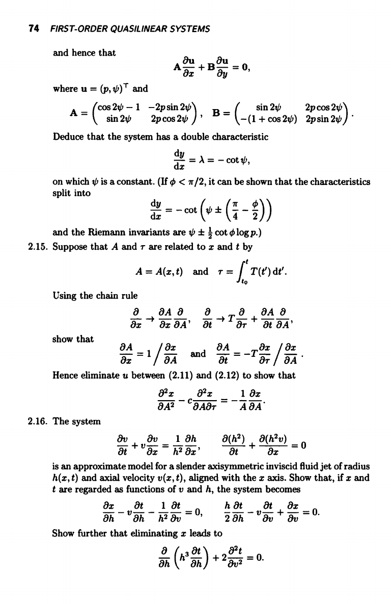
74 FIRST-ORDER QUASILINEAR SYSTEMS
and hence that
where u = (p, ,')' and
_ cos 2t' - I -2p sin
sin 2t/i
2p cos 2t'
A
sin 20
2p cos 2 , '
B
- -(1 + cos 20) 2p sin 21 '
Deduce that the system has a double characteristic
dx =
A
= -
cot t',
on which t¢ is a constant. (If ¢ < 7r/2, it can be shown that the characteristics
split into
ax =
-cot
\OA: (4
2) )
and the Riemann invariants are t/' ± 1 cot 0logp.)
2.15. Suppose that A and r are related to x and t by
j
A = A(x, t)
and
r = T (t') dt'.
o
Using the chain rule
8
-"
8x 8A' a
-+ T
8 + 8t 8A'
show that
OA
8x 8A _ 8z
8x
8x
1 8A
and
at
-Tax
/0A
Hence eliminate u between (2.11) and (2.12) to show that
82x 82x _ 1 8x
8A2 8A8r
A 8A
2.16. The system
8v 8v
=
1 Oh
8(h2) 8(h2v) _
8t +
v
8x h2 8x' 8t + 8x = 0
is an approximate model for a slender axisymmetric inviscid fluid jet of radius
h(x, t) and axial velocity v(x, t), aligned with the x axis. Show that, if x and
t are regarded as functions of v and h, the system becomes
8x at
1 at
h at
8t 8x
Y h-
v 8h
_
ha 8;
_
0'
2 8h
- v - + - = 0 .
Show further that eliminating x leads to
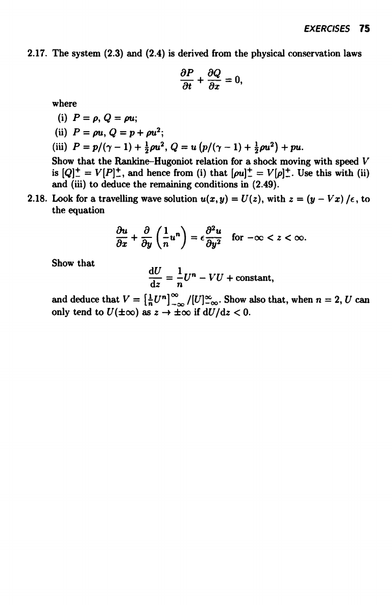
EXERCISES 75
2.17. The system (2.3) and (2.4) is derived from the physical conservation laws
OP N
aP+OQ=0
where
(i) P=P,Q=Pu;
(u) P = Pu, Q = P + Pu2;
(iii) P=p/(7-1)+2Pu2,Q=u(p/(7-1)+2pu2)+pu.
Show that the Rankine-Hugoniot relation for a shock moving with speed V
is [Q]± = V [P]+-, and hence from (i) that [pu]± = V [p]+-. Use this with (ii)
and (iii) to deduce the remaining conditions in (2.49).
2.18. Look for a travelling wave solution u(x, y) = U(z), with z = (y - Vx) /E, to
the equation
- (1 \
8x+- nuJ
02u
= E aye
for -oc < z < oo.
Show that
T z-
U" - VU + constant,
and deduce that V = [nU"] oo /[. Show also that, when n = 2, U can
only tend to U(±oo) as z -> too if dU/dz < 0.
3
Introduction to second-order
scalar equations
3.1
Preamble
In Chapter 2 we tried to describe, in the simplest possible terms, the only reason-
ably general framework that exists concerning the solutions of the Cauchy problem
for arbitrary partial differential equations. Many pages could now be spent in ex-
plaining this framework in more detail, but we will instead devote the next three
chapters to a more specialised analysis of three commonly occurring classes of
second-order scalar equations. This will enable us not only to illustrate as simply
as possible the subtleties that can arise when 'non-hyperbolic' equations are being
solved, but also to look at the role played by the ideas proposed in Chapter 2 when
they are viewed in a more concrete setting.
When we start to consider specific second-order equations in Chapters 4-6,
we will find that we rapidly encounter formidable technical difficulties. Hence this
chapter is a preface that emphasises the central ideas that will need to be kept in
mind in the next three chapters.
Before we start, let us make one elementary observation to illustrate the care
that may have to be taken with what appear to be harmless enough second-order
scalar equations. It comes from a trivial piece of Fourier analysis and shows that the
qualitative behaviour of the solutions of second-order partial differential equations
with Cauchy data is far more diverse than in the case for initial value problems
for second-order ordinary differential equations. In the latter case, the Cauchy-
Picard theorem guarantees existence, uniqueness and continuous dependence on
the data, assuming only appropriate Lipschitz continuity. However, we shall see
that partial differential equations which are on the face of it much smoother can
in fact lose the property of continuous dependence on the Cauchy data. This fact,
which provides one of the basic motivations for trying to classify these partial
differential equations, is illustrated by considering the solutions of the two problems
(i)
au 02u
=
(3.1)
(ii)
8y
Ox2'
2--
8 22
(3.2)
in y > 0, with data
76
PREAMBLE 77
u(x, 0) _ E an cosnx
for -oo
< x
< oo.
(3.3)
n=0
We assume that an are such that u(x, 0) has continuous second derivatives, which
clearly demands that an = o(n-2) as n -a co.
Separation of the variables gives the respective solutions as
00
/
(i) u =
r `ane-nzYCosnx,
n=0
00
(ii) u = E
n2 N
Cos nx.
n=0
The series (3.4) has better convergence properties than (3.3) for y > 0, but the
series (3.5) does not even converge unless an decays very rapidly indeed as n -* oo.
For example, even if an = e-"', (3.5) blows up as y -* 1 (if an = e-`"3, f > 0,
blow-up is at y = e, however small that may be, and if an = O(e-`"), as is generic
for periodic analytic functions, there is no solution at all).
Similarly, if we consider the problems
02U
2 =
8zx2
, (3.6)
a
(iv)
802U 0
yz
8x2
(3.7)
for y > 0, with, for example, data
u(x, 0) = E a. cos nx,
00
n=0
the Fourier series solutions are
(iii)
E an cos ny cos nx,
n=0
8U
(x, 0) = 0,
00
E an cosh ny Cos nx,
n=0
(3.10)
respectively, and a similar contrast can be drawn to that between (3.4) and (3.5).
The switch from (3.6) to (3.7) can easily occur in practice, as has been an-
ticipated on p.42. Suppose that we have an `irrotational' solution of the system
(2.8)-(2.10) describing linearised steady gas dynamics, so that (6i, u) = V O. Elim-
inating p gives
U al
a z
((
\1-
/8x2+Oy2-0;
(3.11)
depending whether the Mach number U/ao is greater or less than unity, we are
effectively led to (3.6) or (3.7), respectively. In fact, the derivation of (3.11) breaks
