Ockendon J., Howison S., Lacey A., Movchan A. Applied Partial Differential Equations

Подождите немного. Документ загружается.

INTRODUCTION TO SECOND-ORDER SCALAR EQUATIONS

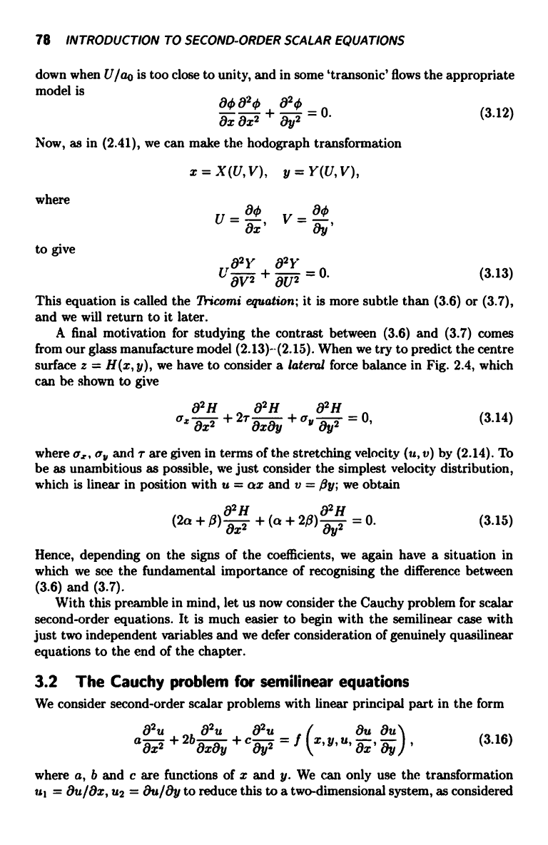
down when U/ao is too close to unity, and in some `transonic' flows the appropriate

model is

Now, as in (2.41), we can

where

to give

006,10

a2q

ax axe

gy2 -

make the hodograph transformation

x = X (U, V ),

y = Y(U, V),

ax00 '

ay,

(3.12)

02y

a2y

(J.

+ aU2 = 0.

(3.13)

This equation is called the Picomi equation; it is more subtle than (3.6) or (3.7),

and we will return to it later.

A final motivation for studying the contrast between (3.6) and (3.7) comes

from our glass manufacture model (2.13)--(2.15). When we try to predict the centre

surface z = H(x, y), we have to consider a lateral force balance in Fig. 2.4, which

can be shown to give

z H

02H

02 H

ax 82 + 27 8ay + ay

= 0,

(3.14)

where or, a and r are given in terms of the stretching velocity (u, v) by (2.14). To

be as unambitious as possible, we just consider the simplest velocity distribution,

which is linear in position with u = ax and v =,6y; we obtain

02H

(2a+0)

+(a+2f)8H2 =

(3.15)

Hence, depending on the signs of the coefficients, we again have a situation in

which we see the fundamental importance of recognising the difference between

(3.6) and (3.7).

With this preamble in mind, let us now consider the Cauchy problem for scalar

second-order equations. It is much easier to begin with the semilinear case with

just two independent variables and we defer consideration of genuinely quasilinear

equations to the end of the chapter.

3.2

The Cauchy problem for semilinear equations

We consider second-order scalar problems with linear principal part in the form

2 2

02U

2baxay + C

= f

(x,

y, u,

8x,

21j)

(3.16)

where a, b and c are functions of x and y. We can only use the transformation

ul = Ou/ax, U2 = Ou/ay to reduce this to a two-dimensional system, as considered

THE CAUCHY PROBLEM FOR SEMILINEAR EQUATIONS 79

in Chapter 2, when the right-hand side of this equation does not depend on u

(otherwise the resulting system is three-by-three). If this can be done, appropriate

Cauchy boundary data would be for ul and u2 to be given on some curve I' in

the (x, y) plane. However, even when f depends on u, it is reasonable to consider

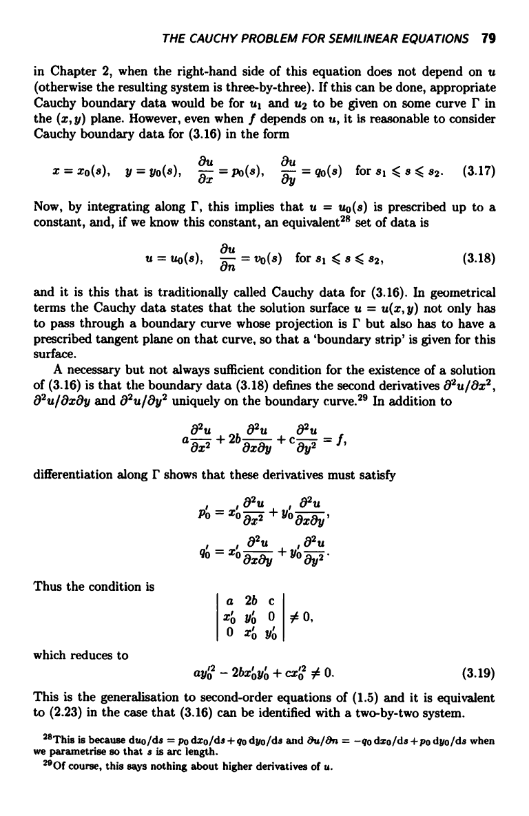
Cauchy boundary data for (3.16) in the form

x = xo(s), y = yo(s),

8x = PO(s), a = q0(s)

forsl <8<82.

(3.17)

Now, by integrating along r, this implies that u = uo(s) is prescribed up to a

constant, and, if we know this constant, an equivalent2s set of data is

= vo(s)

for sl < 8 < 82i

(3.18)

u = uo(8),

and it is this that is traditionally called Cauchy data for (3.16). In geometrical

terms the Cauchy data states that the solution surface u = u(x, y) not only has

to pass through a boundary curve whose projection is r but also has to have a

prescribed tangent plane on that curve, so that a `boundary strip' is given for this

surface.

A necessary but not always sufficient condition for the existence of a solution

of (3.16) is that the boundary data (3.18) defines the second derivatives 82u/8x2,

6'u/OxOy and 82u/8y2 uniquely on the boundary curve.29 In addition to

02u

+26-x8 +c8 uu

= f,

z y y2

differentiation along r shows that these derivatives must satisfy

02u

82u

A =

8x2

y0 8x8y,

82u

02u

y° 8y2 .

8x8y

Thus the condition is

2b c

xo l

# 0,

which reduces to

0 xo yo

ayo - 2bxoyo + cxo

0. (3.19)

This is the generalisation to second-order equations of (1.5) and it is equivalent

to (2.23) in the case that (3.16) can be identified with a two-by-two system.

28This is because duo/da = po dxo/ds+qo dyo/ds and 8u/8n = -qodxo/ds+po dyo/da when

we parametrise so that a is arc length.

Of course, this says nothing about higher derivatives of u.

80 INTRODUCTION TO SECOND-ORDERSCALAR EQUATIONS

3.3

Characteristics

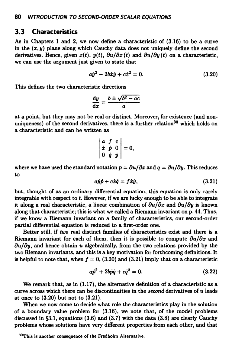
As in Chapters 1 and 2, we now define a characteristic of (3.16) to be a curve

in the (z, y) plane along which Cauchy data does not uniquely define the second

derivatives. Hence, given x(t), y(t), Ou/Ox (t) and Ou/8y (t) on a characteristic,

we can use the argument just given to state that

aye-2b4+C22=0.

This defines the two characteristic directions

dy bf b --ac

dx a

(3.20)

at a point, but they may not be real or distinct. Moreover, for existence (and non-

uniqueness) of the second derivatives, there is a further relation30 which holds on

a characteristic and can be written as

a f c

x P 0

0qy

= 0,

where we have used the standard notation p = Ou/8x and q = Ou/Oy. This reduces

aye + ciq = f4,

(3.21)

but, thought of as an ordinary differential equation, this equation is only rarely

integrable with respect to t. However, if we are lucky enough to be able to integrate

it along a real characteristic, a linear combination of Ou/8z and Ou/Oy is known

along that characteristic; this is what we called a Riemann invariant on p. 44. Thus,

if we know a Riemann invariant on a family of characteristics, our second-order

partial differential equation is reduced to a first-order one.

Better still, if two real distinct families of characteristics exist and there is a

Riemann invariant for each of them, then it is possible to compute 8u/8z and

Ou/Oy, and hence obtain u algebraically, from the two relations provided by the

two Riemann invariants, and this is a key motivation for forthcoming definitions. It

is helpful to note that, when f = 0, (3.20) and (3.21) imply that on a characteristic

aP2

+ 2b0¢ + c42 = 0. (3.22)

We remark that, as in (1.17), the alternative definition of a characteristic as a

curve across which there can be discontinuities in the second derivatives of u leads

at once to (3.20) but not to (3.21).

When we now come to decide what role the characteristics play in the solution

of a boundary value problem for (3.16), we note that, of the model problems

discussed in §3.1, equations (3.6) and (3.7) with the data (3.8) are clearly Cauchy

problems whose solutions have very different properties from each other, and that

30This is another consequence of the Fredholm Alternative.

CHARACTERISTICS 81

(3.6) has real characteristics while (3.7) does not. We also note that (3.1) and (3.2)

have the attributes of a Cauchy problem in that there are as many pieces of data

as there are y derivatives in the partial differential equations, and that they have

coincident real characteristics y = constant. A picture of how we should classify

equations such as (3.16) is now emerging, and corroboration is provided by noting

what happens to (3.16) if we change coordinates with the dual aim of identifying

invariant properties of the left-hand side of the equation and, if possible, writing

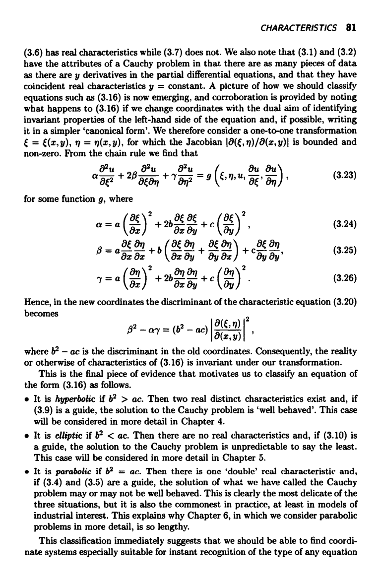
it in a simpler `canonical form'. We therefore consider a one-to-one transformation

C = C(x, y), q = rl(x, y), for which the Jacobian I8(e, n))/8(x, y)I is bounded and

non-zero. From the chain rule we find that

822

82u

= g (C,

8u 8u1

(3.23)

for some function g, where

/ \

= Q

\OX/2

+2b

Oxt9y \8y)

=a8-8--+b(a22+8-8q/ +cLt&I,

OX ex

8x 8y 8y ax / 8y 8y

")2

+ 2b

all Z'hl

(3.24)

(3.25)

(3.26)

Hence, in the new coordinates the discriminant of the characteristic equation (3.20)

becomes

02-Q')'=(b2-aC)IO

,rI)I

8(x,y)

where b2 - ac is the discriminant in the old coordinates. Consequently, the reality

or otherwise of characteristics of (3.16) is invariant under our transformation.

This is the final piece of evidence that motivates us to classify an equation of

the form (3.16) as follows.

It is hyperbolic if b2 > ac. Then two real distinct characteristics exist and, if

(3.9) is a guide, the solution to the Cauchy problem is `well behaved'. This case

will be considered in more detail in Chapter 4.

It is elliptic if b2 < ac. Then there are no real characteristics and, if (3.10) is

a guide, the solution to the Cauchy problem is unpredictable to say the least.

This case will be considered in more detail in Chapter 5.

It is parabolic if b2 = ac. Then there is one `double' real characteristic and,

if (3.4) and (3.5) are a guide, the solution of what we have called the Cauchy

problem may or may not be well behaved. This is clearly the most delicate of the

three situations, but it is also the commonest in practice, at least in models of

industrial interest. This explains why Chapter 6, in which we consider parabolic

problems in more detail, is so lengthy.

This classification immediately suggests that we should be able to find coordi-

nate systems especially suitable for instant recognition of the type of any equation

82 INTRODUCTION TO SECOND-ORDER

SCALAR EQUATIONS

of the form (3.16), and we will indeed find such canonical forms shortly. However,

let us first digress to note that the practical examples mentioned in §3.1 suggest

some models that have the unfortunate property of being of mixed type, that is

they may be hyperbolic in some region in the (x, y) plane and elliptic in others.

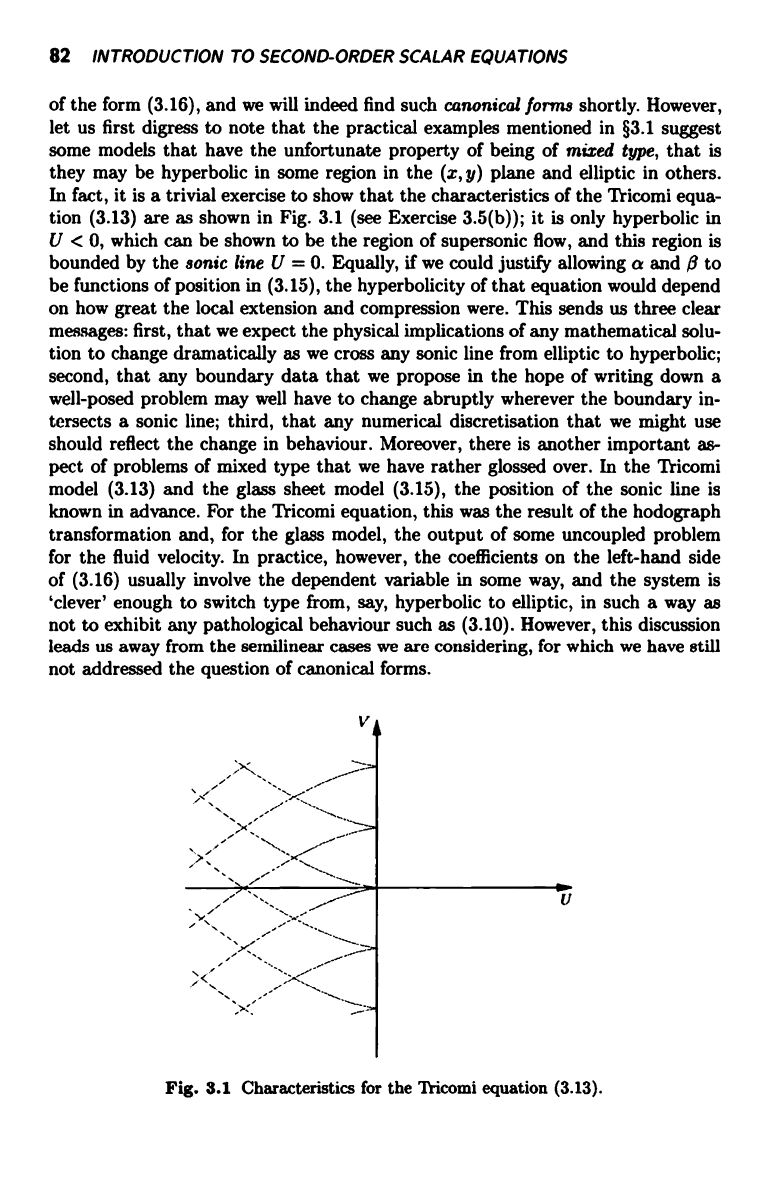
In fact, it is a trivial exercise to show that the characteristics of the Tricomi equa-

tion (3.13) are as shown in Fig. 3.1 (see Exercise 3.5(b)); it is only hyperbolic in

U < 0, which can be shown to be the region of supersonic flow, and this region is

bounded by the sonic line U = 0. Equally, if we could justify allowing a and 6 to

be functions of position in (3.15), the hyperbolicity of that equation would depend

on how great the local extension and compression were. This sends us three clear

messages: first, that we expect the physical implications of any mathematical solu-

tion to change dramatically as we cross any sonic line from elliptic to hyperbolic;

second, that any boundary data that we propose in the hope of writing down a

well-posed problem may well have to change abruptly wherever the boundary in-

tersects a sonic line; third, that any numerical discretisation that we might use

should reflect the change in behaviour. Moreover, there is another important as-

pect of problems of mixed type that we have rather glossed over. In the Tricomi

model (3.13) and the glass sheet model (3.15), the position of the sonic line is

known in advance. For the Tlicomi equation, this was the result of the hodograph

transformation and, for the glass model, the output of some uncoupled problem

for the fluid velocity. In practice, however, the coefficients on the left-hand side

of (3.16) usually involve the dependent variable in some way, and the system is

`clever' enough to switch type from, say, hyperbolic to elliptic, in such a way as

not to exhibit any pathological behaviour such as (3.10). However, this discussion

leads us away from the se:nilinear cases we are considering, for which we have still

not addressed the question of canonical forms.

Fig. 3.1 Characteristics for the Tricomi equation (3.13).

CANONICAL FORMS FOR SEMILINEAR EQUATIONS 83

3.4

Canonical forms for semilinear equations

3.4.1

Hyperbolic equations

When the equation

82u 82u 82u

f (

8u 8u

a 8x2 + 2b

8x8y

+ caye =

x, y, u,

8x ,

is hyperbolic, two real characteristic directions exist at each point and define two

distinct families of characteristics. Now, assuming Lipschitz continuity conditions

on a, b and c, the characteristic condition (3.20), aye - 2bi) + cat = 0, is a pair of

ordinary differential equations for which integrals certainly exist, although it may

not be possible to write them down explicitly. Thus two characteristic variables

may be defined, constant values of one variable giving one characteristic family,

and constant values of the second variable giving the other. Such a definition is not

unique, since any well-behaved function of a characteristic variable thus defined

would also be a characteristic variable, and hence, in practice, such variables are

often chosen aesthetically. All that is necessary is that we choose l and rI in (3.23) so

that t (x, y) = constant and r7(x, y) = constant are in fact the integral curves of the

characteristic equations.31 Now, on 1:(x, y) = constant, (8£/8x).i + (8i;/8y)y = 0,

with a similar relation on 77(x, y) = constant. Substituting into (3.20), we find that

(81;/8x) / (81:/8y) and (8r7/8x) / (8q/8y) are the two (real and distinct) roots of

aa2 + 2bA + c = 0.

(3.27)

Hence, in (3.24)-(3.26), a = 7 = 0. Also

20=a(8f

+491)2+2b(L

+ i'

8x 8x 8x Oy

8y 8y 8y

and this quantity is non-zero since (3.27) only has two roots for A. Thus a hyper-

bolic equation has the canonical form

Ft2;

= G

t, rJ, u, 8t , 8

)

(3.28)

Different choices of characteristic variables merely lead to different right-hand sides

in this equation.

Example 3.1 (The wave equation) A very well-studied example leading to (3.28)

a° axe - aye = f (x, y), ao = constant, (3.29)

which, when f = 0, is referred to as the wave equation. The characteristics are given

by aoy2 = *2 and the problem is hyperbolic; one particular choice of characteristic

31This distinction is related to our discussion of the representation of characteristics in §§1.8

and 2.6.

INTRODUCTION TO SECOND-ORDER SCALAR EQUATIONS

variables is t = x - aoy and n = x + aoy. It is easily verified that a = ry = 0 and

,6 = 2ao, so that a canonical form is, say,

.9tN

4a02 f

n' 2ao)

= n)

(3.30)

This example reveals one of the benefits that can occasionally accrue from writ-

ing the equation in canonical form; it actually enables us to perform an explicit

integration to give the general solution of (3.30) as the d'Alembert representation

u =

Jf9(eii) d do + hl (t) + h2(n),

(3.31)

where hl and h2 are arbitrary functions to be determined by the boundary condi-

tions. Alternatively, we could have derived this formula by integrating (3.29) along

the characteristics to give the R.iemann invariants

fan

f/dy

on x

aoy = constant. (3.32)

Example 3.2 Things are not usually so easy, as can be seen by considering

8x2 -

8y82

22 = 0.

(3.33)

The characteristics are given by yy = ±xi, and the equation is hyperbolic except

on the axes where x = 0 or y = 0, which we exclude from the domain of interest.

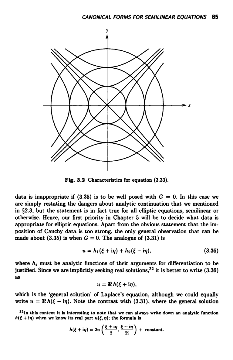
Characteristic variables are given by t = y2 - x2 and n = x2 + y2, and the two

families of characteristics are shown in Fig. 3.2; note that they touch on the axes.

A tedious calculation leads to

82u

Lou

at-

2(q2 -

t2) 8n 8t) (3.34)

which is in canonical form, but there are no Riemann invariants, and neither can

(3.34) be integrated explicitly.

3.4.2 Elliptic equations

In the elliptic case, real characteristic variables no longer exist and the integrals

of (3.20) are complex conjugate pairs of functions y(x). We choose f and n to

be the real and imaginary parts of these complex integrals so that the `complex'

characteristics are Z; tin = constant, and (8£/8x±iO /8x)x+(8{/8y±i8n/8y)y =

0. Substituting into (3.23) and taking real and imaginary parts we obtain a = ry

0 and 3 = 0. The canonical form is therefore

z02U

n22

= G

(to?,

u, , 8 )

(3.35)

When G = 0, this equation is called Laplace's equation. The Cauchy-Riemann

system on p. 46 and the example (3.7) and (3.8) both show that Cauchy boundary

CANONICAL FORMS FOR SEMILINEAR EQUATIONS 85

Fig. 3.2 Characteristics for equation (3.33).

data is inappropriate if (3.35) is to be well posed with G = 0. In this case we

are simply restating the dangers about analytic continuation that we mentioned

in §2.3, but the statement is in fact true for all elliptic equations, semilinear or

otherwise. Hence, our first priority in Chapter 5 will be to decide what data is

appropriate for elliptic equations. Apart from the obvious statement that the im-

position of Cauchy data is too strong, the only general observation that can be

made about (3.35) is when G = 0. The analogue of (3.31) is

u = hl (£ + ir)) + h2V - iq),

(3.36)

where hi must be analytic functions of their arguments for differentiation to be

justified. Since we are implicitly seeking real solutions,32 it is better to write (3.36)

u = R h( + iq),

which is the `general solution' of Laplace's equation, although we could equally

write u = 9 h(£ - hp). Note the contrast with (3.31), where the general solution

321n this context it is interesting to note that we can always write down

an analytic function

h(( + iq) when we know its real part u(f, q); the formula is

h(f + iq) = 2u

i", 4

1 + constant.

INTRODUCTION TO SECOND-ORDER SCALAR EQUATIONS

involved two twice-differentiable functions rather than one analytic one. Not sur-

prisingly, the theory of functions of a complex variable is intimately related to the

solution of Laplace's equation in llt2 and Chapter 5 provides several illustrations

of how this theory can be put to practical use.

3.4.3 Parabolic equations

In the parabolic case, the characteristic equation (3.20) has a double root and

there is only one real characteristic variable. If we choose q to be this variable,

so that (8q/8x)i + (8q/8y)y = 0, then, on substituting into (3.26), ry = 0. As

always, there is some freedom of choice for a and, if a # 0, we may conveniently

choose t = x so that a = a (if a = 0 we choose

= y, since then c 0 0). But

ry = (a 8q/8x + b 8q/8y)2/ a = #2 /a and hence ft

=\ 0. The canonical form is thus

8 22 = G

\t, q, u,

8t , aq

(3.37)

The subtlety of this case is illustrated by contrasting the parabolic equations

0 and 82u/8t2 = 8u/8q. The former, although trivial, behaves like

a hyperbolic equation because the general solution is t f (q) + g(q), where f and

g are arbitrary, and hence this solution is uniquely defined by Cauchy data on

any non-characteristic, i.e. any line excluding q = constant;33 the latter, which is

called the diffusion equation or heat equation, is so complicated as to occupy much

of Chapter 6.

We remark that, as often happens in applied mathematics, degenerate cases

are best understood by taking judiciously chosen limits of non-degenerate ones.

Here, a good idea of the kind of data that should be applied to parabolic equations

can be gleaned from the limit of the hyperbolic equation

8-e2

(3.38)

as a -a 0. This equation is an example of what will be studied in Chapter 4 as the

telegraph equation; its characteristics are q f of = constant, and we expect that

well-posed data would be, for example, the prescription

u = f (0, = g(f) )

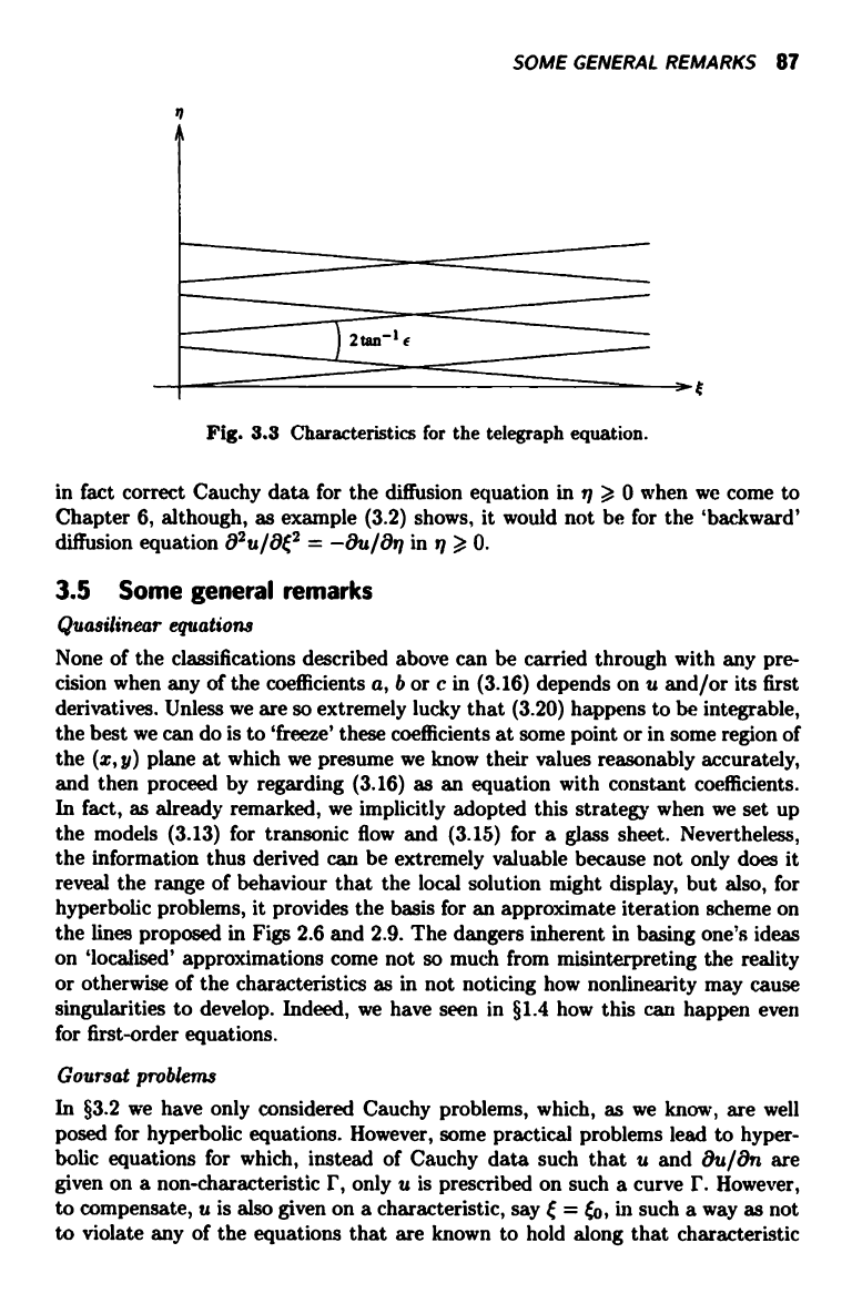
on the non-characteristic q = 0. However, the characteristics are shown in Fig. 3.3,

suggesting that u may change much more rapidly in the q direction than in the

direction. In fact, if we neglect t derivatives altogether in (3.38), we obtain the

approximation 34

u rs f (0 -

which suggests that, when q is much bigger than e, the solution has 'forgotten'

about g(i;) and only remembers the data u = f

We will verify that u = f is

"Recall that we have seen in §§2.4.2 and 2.4.3 that systems with a double characteristic can

exhibit the structure of hyperbolic systems.

34 Technically, there is a 'boundary layer' on q = 0.

SOME GENERAL REMARKS 87

2tan- I F

Fig. 3.3 Characteristics for the telegraph equation.

in fact correct Cauchy data for the diffusion equation in rl > 0 when we come to

Chapter 6, although, as example (3.2) shows, it would not be for the `backward'

diffusion equation 82u/81;2 = -8u/8q in t' > 0.

3.5

Some general remarks

Quasilinear equations

None of the classifications described above can be carried through with any pre-

cision when any of the coefficients a, b or c in (3.16) depends on u and/or its first

derivatives. Unless we are so extremely lucky that (3.20) happens to be integrable,

the best we can do is to `freeze' these coefficients at some point or in some region of

the (x, y) plane at which we presume we know their values reasonably accurately,

and then proceed by regarding (3.16) as an equation with constant coefficients.

In fact, as already remarked, we implicitly adopted this strategy when we set up

the models (3.13) for transonic flow and (3.15) for a glass sheet. Nevertheless,

the information thus derived can be extremely valuable because not only does it

reveal the range of behaviour that the local solution might display, but also, for

hyperbolic problems, it provides the basis for an approximate iteration scheme on

the lines proposed in Figs 2.6 and 2.9. The dangers inherent in basing one's ideas

on `localised' approximations come not so much from misinterpreting the reality

or otherwise of the characteristics as in not noticing how nonlinearity may cause

singularities to develop. Indeed, we have seen in §1.4 how this can happen even

for first-order equations.

Goursat problems

In §3.2 we have only considered Cauchy problems, which, as we know, are well

posed for hyperbolic equations. However, some practical problems lead to hyper-

bolic equations for which, instead of Cauchy data such that u and 8u/8n are

given on a non-characteristic r, only u is prescribed on such a curve r. However,

to compensate, u is also given on a characteristic, say s = 60, in such a way as not

to violate any of the equations that are known to hold along that characteristic