Ockendon J., Howison S., Lacey A., Movchan A. Applied Partial Differential Equations

Подождите немного. Документ загружается.

INTRODUCTION TO SECOND-ORDER SCALAR EQUATIONS

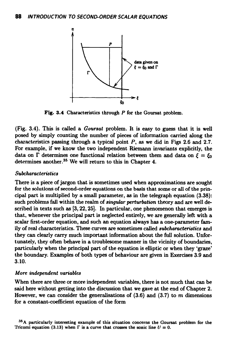
data given on

t=lpandr

Fig. 3.4 Characteristics through P for the Goursat problem.

(Fig. 3.4). This is called a Goursat problem. It is easy to guess that it is well

posed by simply counting the number of pieces of information carried along the

characteristics passing through a typical point P, as we did in Figs 2.6 and 2.7.

For example, if we know the two independent Riemann invariants explicitly, the

data on r determines one functional relation between them and data on

= Co

determines another.35 We will return to this in Chapter 4.

Subcharacteristics

There is a piece of jargon that is sometimes used when approximations are sought

for the solutions of second-order equations on the basis that some or all of the prin-

cipal part is multiplied by a small parameter, as in the telegraph equation (3.38):

such problems fall within the realm of singular perturbation theory and are well de-

scribed in texts such as [3,22, 25]. In particular, one phenomenon that emerges is

that, whenever the principal part is neglected entirely, we are generally left with a

scalar first-order equation, and such an equation always has a one-parameter fam-

ily of real characteristics. These curves are sometimes called subcharacteristics and

they can clearly carry much important information about the full solution. Unfor-

tunately, they often behave in a troublesome manner in the vicinity of boundaries,

particularly when the principal part of the equation is elliptic or when they `graze'

the boundary. Examples of both types of behaviour are given in Exercises 3.9 and

3.10.

More independent variables

When there are three or more independent variables, there is not much that can be

said here without getting into the discussion that we gave at the end of Chapter 2.

However, we can consider the generalisations of (3.6) and (3.7) to m dimensions

for a constant-coefficient equation of the form

35A particularly interesting example of this situation concerns the Coursat problem for the

Tticomi equation (3.13) when r is a curve that crosses the sonic line U = 0.

EXERCISES 89

02U

m-'

C72u

aye

C572

u1Y=0 =

an,...n.,,-i cos(nlxl) ... COS(nm-lxm-l),

can be written as

y-0

- 0,

u =

an,...nm_, cOs(ny) cOS(njx1) ... coS(nm-lxm-1),

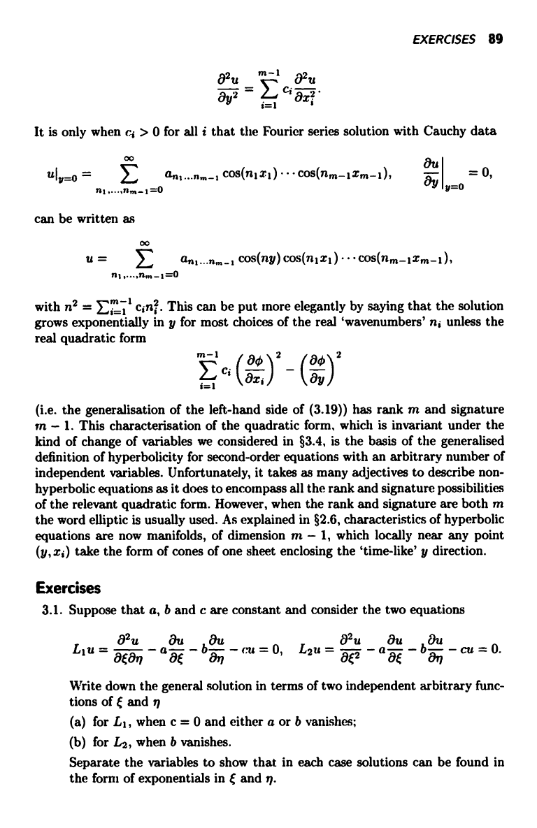
with n2 = E' 1 cin; . This can be put more elegantly by saying that the solution

i__ I

grows exponentially in y for most choices of the real `wavenumbers' ni unless the

real quadratic form

uc8x)z-(9Y

(i.e. the generalisation of the left-hand side of (3.19)) has rank m and signature

m - 1. This characterisation of the quadratic form, which is invariant under the

kind of change of variables we considered in §3.4, is the basis of the generalised

definition of hyperbolicity for second-order equations with an arbitrary number of

independent variables. Unfortunately, it takes as many adjectives to describe non-

hyperbolic equations as it does to encompass all the rank and signature possibilities

of the relevant quadratic form. However, when the rank and signature are both m

the word elliptic is usually used. As explained in §2.6, characteristics of hyperbolic

equations are now manifolds, of dimension m - 1, which locally near any point

(y,xi) take the form of cones of one sheet enclosing the 'time-like' y direction.

Exercises

3.1. Suppose that a, b and c are constant and consider the two equations

L1u=J02U

--a8 -b--eu=0,

L2U=8 -a8,--b

cu=0.

Write down the general solution in terms of two independent arbitrary func-

tions off and rl

(a) for L1, when c = 0 and either a or b vanishes;

(b) for L2, when b vanishes.

Separate the variables to show that in each case solutions can be found in

the form of exponentials in C and rl.

INTRODUCTION TO SECOND-ORDER SCALAR EQUATIONS

3.2. Suppose Dj = aj 8/8x + bj 8/8y + cj, j = 1,

... , 4, where aj, bj and ej are

constant, and

Dju + D2v = 0,

D3u+D4v=0.

Show that u and v satisfy scalar second-order equations whose type depends

on the roots of

det (I aa,

a2 b, b2

3 a4

b3 b4

) )

3.3. Show that the equations

02u 82u

02u 8u 82u 8u

(i)

8x2

= 0,

(ii)

8x2

= u,

(ill)

8x2 = 8x'

(iv)

8xz = aU

can be written as first-order systems for u = (u,v)T, where v = 8u/8x, in

the form

A8x

+B5

=c,

where for cases (i)-(iii)

- (0

0),

' B= (0 0),

and for case (iv)

A=(0 0), B=(O1 Q).

Show further that, when A is such that det(B - AA) = 0, then B - AA

has two linearly independent left eigenvectors in cases (i)-(iii), but only one

in case (iv). Show also that (i)-(iii) can usually be made to satisfy Cauchy

data, but that (iv) cannot.

3.4. By transforming to canonical form, show that the general solution of

02U

z z

8x22 + 3 8x8y + ayz

+ sin

(x + y) = 0

is u = f (x - 3y) + g(y - 3x) + 18 sin (x + y), where f and g are arbitrary.

3.5. Show that the Ticomi-type equations

z z

( ) + 0a

8x2 8y2 '

02u 02u

(b)

-y8x2 + 8y2 = 0,

( )

- z

8xz

EXERCISES 91

are hyperbolic in x < 0, y > 0 and x # 0, respectively, and that characteristic

coordinates are

(a)

= y +

2(-x)12,

*I = y -

2(-x)112,

(b)

=3x+2y312,

n=3x-2y312,

(c)

=y+loglxl, 7i=y-loglxl.

Sketch the characteristics in each case and show that the corresponding

canonical forms are

(a)

(b)

(c)

3.6. Show that, if

(L-

) /2(q -

/6(t- n),

02U

OU au

- -)/4.

8017 0% at

82u 82u

(x + ay) axe + aye = 0,

where a i4 0, the characteristics are given by

(z ± a)2 4az + 2a2 log(z ± a) + x = constant,

where z2 = x + ay. Show that, for small z, the characteristics through the

origin are

(x + ay)3/2 =

3ax

What happens if a = 0?

3.7. Show that the equation

2x2

axe

+ 5xy

8x.y +

2y2 8-2 + 8x 8- + 5y

= 0

is hyperbolic and that characteristic coordinates are = x2/y and q = y2/x.

Giving yourself lots of time, show that the canonical form is

02U

= 0,

and hence that the general solution is u(t, q) = f (t)/q+g(iI), where f and g

are arbitrary. Hence, or otherwise, when u(1, y) = y2 and 8u/8x (1, y) = 1,

show that

1 (2

2 +

7y2

U(-T'

;77

92 INTRODUCTION TO SECOND-ORDER SCALAR EQUATIONS

3.8. Show that, when u(x,0) = uo(x) and Ou/Ot (x, 0) = vo(x), the d'Alembert

representation (3.31) gives

x+aot

u(x, t) = 2 (uo(x - aot) + uo(x + aot)) +

vo(s) d8.

t Opt

3.9. Show that constants a and b can be chosen so that u = ay +

bye-y''

satisfies

02U

49U

+-p+-=0 for-1<x<1,

e1 -

OX2 9y2

with u(1, y) = y and u(-1, y) = -y. Check that, as a -4 0+, u becomes

constant on the subcharacteristics y = constant and satisfies one boundary

condition, but not the other. What happens when a -+ 0-?

3.10. Suppose that u(x, y, t) satisfies the elliptic equation

O2 +f2

02U

0 for0<y<1,

with

ay (x, 0, t) = 0, a (x, 1, t) + e2 5i2 (x, 1, t) = 0.

Show that a formal power series in which

u = uo(x,y,t) + e2u1(x,y,t) + ...

satisfies the equation and boundary condition up to terms of O(e2) if

uo = uo(x,t),

where uo satisfies the hyperbolic equation

0-2U0

O2uo

= 0

ax2 &2

This example, which is a simple model for the tides, shows that the solution

of an elliptic equation can sometimes be consistently approximated by that

of a hyperbolic equation.

Hyperbolic equations

4.1 Introduction

Hyperbolic equations are the easiest scalar second-order equations to classify from

the point of view of the Cauchy problem. They occur commonly in practical appli-

cations, as is evident from studying the models of Chapter 2. Take, for example,

fluid dynamics. We have already remarked in Chapter 3 that a large class of

steady two-dimensional supersonic gas flows can be modelled by the hyperbolic

equation (3.11), (1- U2/ao)820/8x2 + 820/8y2 = 0. However, the requisite cross-

differentiation is not possible for evolutionary models such as the shallow water

model (2.1) and (2.2), or the unsteady gas dynamics model (2.3) and (2.4), except

in the frequently occurring acoustic limit in which the fluid is nearly in a state

of rest or uniform motion. Then, a linearisation procedure can be carried out as

on p. 65. For example, when we assume that u and h - ho in (2.1) and (2.2), or

u, p - po and p - po in (2.3) and (2.4), are small enough for their squares to be

negligible, we obtain the hyperbolic one-dimensional wave equation

820 2820

8t2 = ao 8x2

(4.1)

where as = gho or ao = rypa/po, respectively. Here ¢ is any one of the variables

u or h - ho in (2.1) and (2.2), or u, p - po or p - po in (2.3) and (2.4), the

remaining variables being related to 0 by simple linear transformations. Equally,

the regenerator and fluidised bed models (2.17)-(2.20) can be cross-differentiated

to give a constant-coefficient equation of the form

(

aTx

b) I i

t +

cTx

+ d l u = eu, (4.2)

which is clearly hyperbolic and is a version of the telegraph equation mentioned

in §3.4.3; to see this set u = e°:+dev for suitable n and Q.

Multi-space-dimensional versions of such linear scalar second-order equations

are even more relevant for practical problems. Indeed, much of linear acoustics is

governed by

= aS V2ut

HYPERBOLIC EQUATIONS

in two or three space dimensions,36 and we will discuss how the solutions of such

hyperbolic equations depend on dimensionality in §4.6. Still more interesting is

the appearance of vector versions of (4.3), which should really be classified using

the methods of Chapter 2. However, a generalisation of the discussion of §3.4 will

give us enough of a basis to be able to discuss systems such as Maxwell's equations

and the equations of linear elasticity in §4.7.

Our first task in this chapter is to see how the theory for linear scalar second-

order equations in two independent variables can be put to good use. Since we know

that the Cauchy problem for such equations is well posed, we can immediately

set about finding representations of solutions, confident that such representations

make sense and depend continuously on the data. This is the first time in the book

that a general strategy for representing solutions is presented, and it is not the last,

so a careful preamble about the possible procedures and methodology is given in

§4.2. Moreover, there is one analytical technique, that of eigenfunction expansions,

which we review in §4.4 because it is of such importance in this and subsequent

chapters. Most of the rest of this chapter is devoted to the explicit solution of

linear equations, and we leave those few representations that are available for the

solution of nonlinear hyperbolic problems to the brief §4.8.

4.2 Linear equations: the solution to the Cauchy problem

We begin by considering linear equations that have been transformed to charac-

teristic variables (x, y), so that we have to solve

82u

Gu=8x8y+pex+qay+ru=f,

where p, q, r and f are functions of x and y, but not of u or its derivatives. We

take u and Ou/8n (or, equivalently up to a constant, 8u/8x and 8u/8y) to be

prescribed on some open curve r that is nowhere parallel to the characteristics,

which are the x and y axes. For definiteness we only look for the solution on one

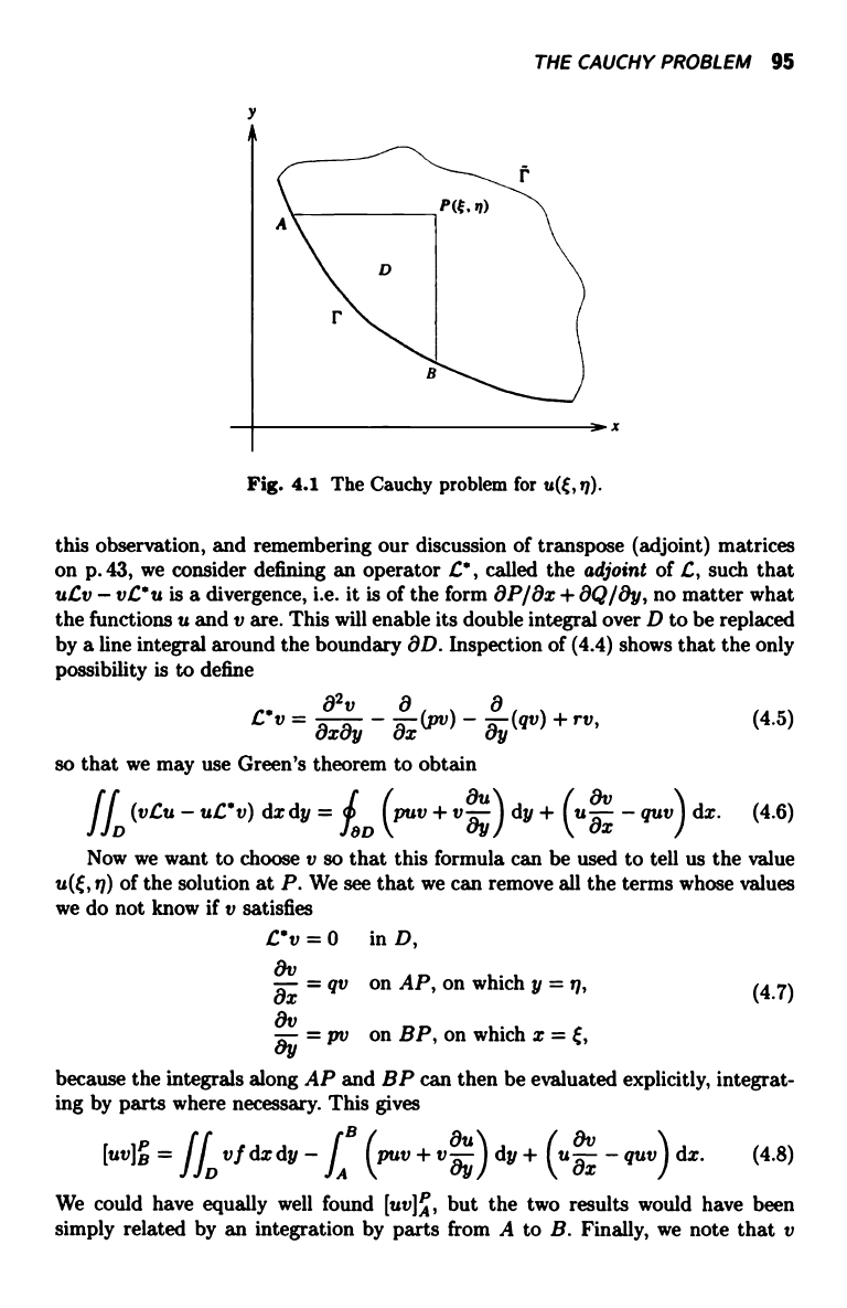
side of this curve, say y increasing, as in Fig. 4.1.

The prescription for the representation for the solution of this general Cauchy

problem can be presented at two different levels and we leave it to the reader to

decide which route to take; they converge at the end of §4.2.2.

4.2.1 An ad hoc approach to Riemann functions

Motivated by §§3.3 and 3.4.1, we ask whether the d'Alembert formula (3.31) could

not be generalised to apply to (4.4). Now the key step in deriving (3.31) was

direct integration with respect to first x and then y, which is one of the many

ways of evaluating a double integral over the region D of Fig. 4.1. In the light of

36Here and henceforth we will use the applied mathematician's notation

_ 82 82

8s2 + 8y2 + 8z2'

where z, y, z denote spatial coordinates.

THE CAUCHY PROBLEM 95

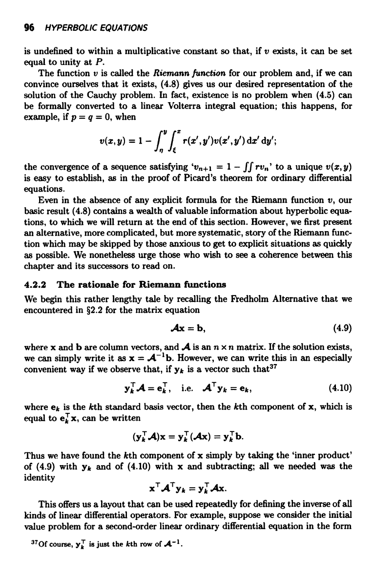
Fig. 4.1 The Cauchy problem for u(C, n).

this observation, and remembering our discussion of transpose (adjoint) matrices

on p. 43, we consider defining an operator C', called the adjoint of C, such that

urv - vC'u is a divergence, i.e. it is of the form OP/8x + 8Q/8y, no matter what

the functions u and v are. This will enable its double integral over D to be replaced

by a line integral around the boundary W. Inspection of (4.4) shows that the only

possibility is to define

Cv =

8 v

(pv) -

(qv) + rv, (4.5)

8x8y ax ay

so that we may use Green's theorem to obtain

\ \

I'D (vCu - uVv) dx dy = illD

+ v

2u-)

dy +

(us!

- quv I dx. (4.6)

Now we want to choose v so that this formula can be used to tell us the value

u(t, p) of the solution at P. We see that we can remove all the terms whose values

we do not know if v satisfies

Vv = 0

in D,

= qv

on AP, on which y = q,

(4.7)

= pv on BP, on which x =

because the integrals along AP and BP can then be evaluated explicitly, integrat-

ing by parts where necessary. This gives

dy +

(u 8-

quv 1 dx. (4.8)

[uv]

= ffD' dx dy -

We could have equally well found [uv]A, but the two results would have been

simply related by an integration by parts from A to B. Finally, we note that v

HYPERBOLIC EQUATIONS

is undefined to within a multiplicative constant so that, if v exists, it can be set

equal to unity at P.

The function v is called the Ricmann function for our problem and, if we can

convince ourselves that it exists, (4.8) gives us our desired representation of the

solution of the Cauchy problem. In fact, existence is no problem when (4.5) can

be formally converted to a linear Volterra integral equation; this happens, for

example, if p = q = 0, when

v(x, y) = 1 - f

f:r

r(x', y')v(x', y') dx' dy';

e convergence of a sequence satisfying

1 - f f

to a unique v(x, y)

is easy to establish, as in the proof of Picard's theorem for ordinary differential

equations.

Even in the absence of any explicit formula for the Riemann function v, our

basic result (4.8) contains a wealth of valuable information about hyperbolic equa-

tions, to which we will return at the end of this section. However, we first present

an alternative, more complicated, but more systematic, story of the Riemann func-

tion which may be skipped by those anxious to get to explicit situations as quickly

as possible. We nonetheless urge those who wish to see a coherence between this

chapter and its successors to read on.

4.2.2 The rationale for Riemann functions

We begin this rather lengthy tale by recalling the Fredholm Alternative that we

encountered in §2.2 for the matrix equation

Ax = b,

(4.9)

where x and b are column vectors, and A is an n x n matrix. If the solution exists,

we can simply write it as x = A-'b. However, we can write this in an especially

convenient way if we observe that, if yk is a vector such that37

Yk A = ek ,

i.e.

ATYk = ek,

(4.10)

where ek is the kth standard basis vector, then the kth component of x, which is

equal to ek x, can be written

(Yk A)x = YT(AX) = Ykb-

Thus we have found the kth component of x simply by taking the `inner product'

of (4.9) with Yk and of (4.10) with x and subtracting; all we needed was the

identity

XTATYk = Yk Ax.

This offers us a layout that can be used repeatedly for defining the inverse of all

kinds of linear differential operators. For example, suppose we consider the initial

value problem for a second-order linear ordinary differential equation in the form

370f course, yk is just the kth row of A.

THE CAUCHY PROBLEM 97

Cu = f(x), C =

i +

P(x)aj + q(x)

for x > 0, (4.11)

with u(0) = du/dx (0) = 0 without loss of generality. We exploit the argument

above by identifying C with A it with x and f with b. We now try to define C,

b, R and an inner product ( , ) so that we can draw the analogies

Ax = b

<-+

Cu(x) = f (x),

u(0) = dZ (0) = 0;

ATYk = ek

++ b(x - l;);

Yk Ax

xTATYk

(R(x,C), Cu(x)) = (u(x), C'R(x,C));

yk b = e,k x H

(R(x, C), f (x)) = (b(x - l), u(x)).

The last line in the left-hand column gives x, component by component, and the

last line in the right-hand column is supposed to give u(t) at all possible values of

C. These analogies will work if we proceed as follows.

1. We define (u(x), v(x)) = f

u(x)v(z) dx for some suitable X > . The motiva-

tion for this is as follows: if we divide the range of integration into N subintervals

of width h, and approximate u(x) and v(z) b y step functions on each subin-

terval, the functions are represented by vectors of values u = (ui , ... , UN) and

v = (vi, ... , vN). The integral of uv is approximated by r uivih = u v h

which, under suitable conditions, becomes f uv dx as N -4 oc.

2. We define

C R = d R - dx (pR) + qR,

which makes uC R - RCu into an exact differential, and in addition we specify

that R(X) = dR/dx (X) = 0.

3. We define b(x - t) to be the so-called delta function, i.e. the limit of a sequence

of well-behaved functions that tend to zero except for very small values of x -1;,

but whose integral over any interval containing x =

is unity. The sequence

could, for example, be defined by

1 _2

b(x) = lim -e =

eto F

(4.12)

By taking limits of integrals of members of this approximating sequence, the

vital result (b(x - {), u(x)) = u(t) in the last line of the analogy can be justified

as long as X >

and, strikingly, it can be shown to follow from limits of any

reasonable sequence of approximating sequences like (4.12).

This last idea is one of the principal motivations for the axiomatic definition of

distributions or generalised functions [37, 42]. In this approach all the `epsilonology'

is swept away by defining the delta function and its relatives as linear functionals

that map a class of suitably smooth test functions to the real numbers 38 We define

The whole philosophy is closely related to that of the theory of weak solutions of hyperbolic

equations in the presence of shock waves, as discussed in §1.7.