Ockendon J., Howison S., Lacey A., Movchan A. Applied Partial Differential Equations

Подождите немного. Документ загружается.

HYPERBOLIC EQUATIONS

this map b y the inner product ( , ); thus, since the inner product of 6(x) and any

well-behaved test function t'(x) is t('(0), we could define 6 axiomatically by the

statement

6(x) :

- ( O ).

In this scenario, any well-behaved function f (x) would be defined as

f(x)'O(x)dx

for all test functions tli, assuming of course that the test functions are such as to

allow the integral to exist. We can go further and define a calculus of distributions

motivated by the formula for integration by parts, which says that

f (x)V,' (x) dx,

f f'(x)G(x) dx

= -

provided that 0 vanishes sufficiently rapidly at x = ±oo. Thus we define 6'(x) by

the rule

(x)o(x) dx f

6(x)0'(x) dx,

f-'0000 6'

so that

6'(x) : 0 -+ -00);

the intuitively obvious statements

6(f)df=H(x)={0,

x<0,

00 111

X>0'

where H(x) is called the Heaviside function, and its consequence

H'(x) = 6(x)

(4.13)

are in accordance with this rule. It can be shown that the delta function, like

all distributions, satisfies the usual rules of calculus, especially that of integration

by parts for the product of a distribution and a smooth function. Moreover, it is

a simple matter to define distributions with, say, two independent variables; for

example, we could either consider 6(x)6(y) to be defined by39

6(x)6(y) = Inn

1e (s+y

E-+o area

or as the functional that takes a test function io(x, y) to 0(0, 0).

It is interesting and important to show that the interpretation of 6(x)6(y) is independent of

any local change of coordinates that preserves area (see Exercise 4.1).

THE CAUCHY PROBLEM 99

At the end of the day, this calculus of distributions, combined with the analogy

above, leads to the solution of (4.11) in the form

uW = / uC*Rdx = J

u(x)8(x - l;) dx

X X

0 o

f RGu dx

= R(x, ) f (x) dx.

The heart of the matter is that Green's theorem (here, integration by parts) can

be used to relate the integrals of uG'R and RCu despite the fact that R has

singularities and that GR is not even a function in the usual sense. Moreover,

noting that R satisfies the linear homogeneous equation C* R = 0 in 1: < x < X,

with R = dR/dx = 0 at x = X, we see that R = 0 for x > . Thus we simply have

u(1;) = R(x, ) f (x) dx.

As a matter of jargon, operators G such that C = G' are called self-adjoint,

and problems for which C = G' and additionally R satisfies the same boundary

conditions as those for u are called self-adjoint problems. Cauchy problems for

hyperbolic equations do not fall into this category, even though C may equal G',

but certain problems for elliptic equations do, as we shall see in Chapter 5. In the

same way that self-adjoint real matrices, i.e. symmetric ones, have real eigenvalues

and orthonormal eigenvectors, so do self-adjoint real differential operators have

real eigenvalues and orthonormal eigenfunctions.

The procedure (4.5)-(4.8) now becomes an obvious generalisation. We simply

define

G'R(x, y; t, n) = 5(x - t)5(y - n)

The nice thing about the layout on p.97 is that, if we now take the boundary

conditions on R as Cauchy data

on any curve outside D (such as I' in Fig. 4.1), we immediately retrieve (4.8)

formally with v = R, G' as in (4.5) and the inner product

uv dx dy.(u(x, y), v(x, y)) = lID

We also note that R =- 0 in the unshaded region between f and D in Fig. 4.1,

because R satisfies homogeneous Cauchy data on I'.

However, the argument above raises a much more subtle question about the

nature of the Riemann function. Since R describes the response of a hyperbolic

equation to an `impulse' at x = t, y = 77, our general arguments about charac-

teristics lead us to expect that R vanishes except in x < t, y < rl, and suffers

100

HYPERBOLIC EQUATIONS

discontinuities of some sort on x = , y < 71, and on y = q, x <

(i.e. BP and

AP, respectively, in Fig. 4.1). But what can we say about these discontinuities?

This is a difficult question whose answer demands that we first look at R in the

vicinity of x = , y = 97. Here, we expect the largest term in V R to be the highest

derivative 82R/8x Oy and, by direct integration and the use of (4.13),

82R

= b(x - C)8(y - rl) implies

R = H(C - x)H(n - y);

that is, locally near x = £, y = q, R is unity in the quadrant x < £, y < q, and

zero outside. Note that this confirms that, as we approach P from inside D, R

tends to unity in accordance with the statement after (4.8).

Now, since R suffers jumps across x = C and y = n locally near P, we expect

from arguments such as those in §1.6 that these jumps persist although they may

change in strength, depending on the form of C. To find these changes, say across

x = {, we note that when we formally integrate C'R = 0 with respect to x across

BP we find

8R -{+0

==f+o -

[pR}==C-o

x={-0

But R_0onx= + 0 so, as we approach x =

from D,

- pR

_ 0,

in accordance with (4.7). The same kind of argument applies on AP.

We thus have achieved a complete agreement between our constructive ap.

proach to the Riemann function and the ad hoc approach of §4.2.1. While §4.2.1

may seem the easier, we will find that the hard work of this section will pay hand-

some dividends in the remaining chapters and especially at the end of Chapter 9.

4.2.3

Implications of the Riemann function representation

From now on we will reserve the notation R for the Riemann function so that (4.8)

becomes

(R+

u(P) - u(B) = J J Rf dx dy j

RJ dy +

- quR I dx.

JJ A /

6iT

(4.14)

We remember that we could have written down a similar formula for u(P) - u(A)

and used it with (4.14) to derive the d'Alembert formula (3.31). We cannot write

down an explicit expression for R for the general hyperbolic equation (4.4), al-

though some examples where this is possible are given below. Nevertheless, the

existence of this function R, which is defined independently of the boundary data

and only depends on the differential operator, gives valuable qualitative informa-

tion about the solution of (4.4) which we summarise below.

1. The solution only depends on the Cauchy data between A and B, where the

characteristics through P meet the boundary curve, and the values of f in D,

the region between the two characteristics through P and the boundary curve.

This region is called the domain of dependence of P, as shaded in Fig. 4.1.

THE CAUCHY PROBLEM 101

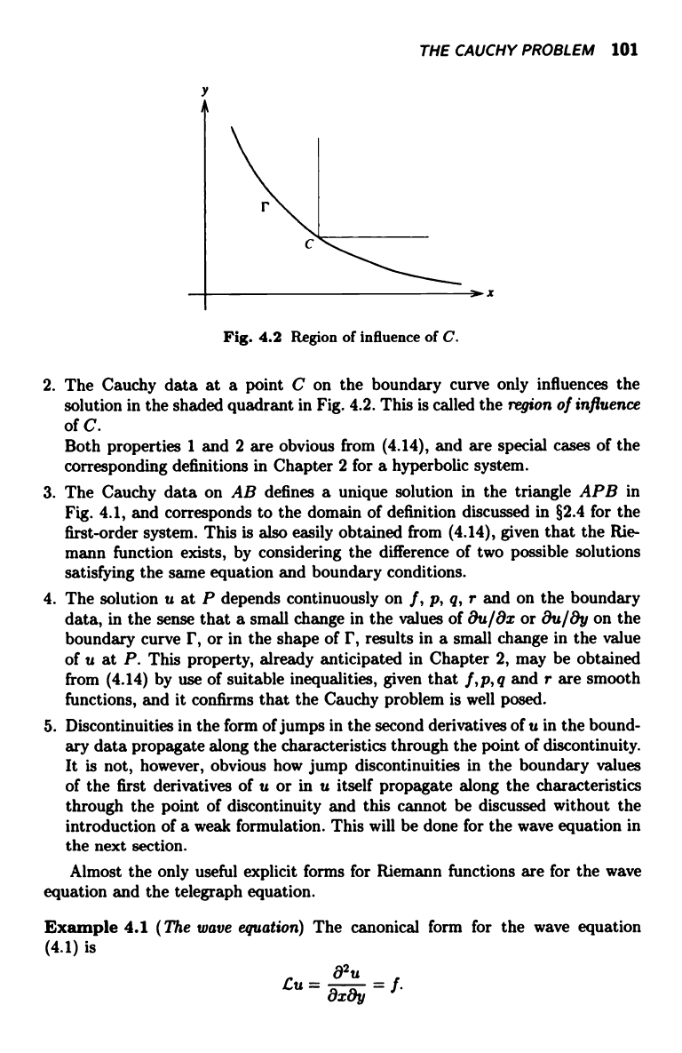
Fig. 4.2 Region of influence of C.

2. The Cauchy data at a point C on the boundary curve only influences the

solution in the shaded quadrant in Fig. 4.2. This is called the region of influence

of C.

Both properties 1 and 2 are obvious from (4.14), and are special cases of the

corresponding definitions in Chapter 2 for a hyperbolic system.

3. The Cauchy data on AB defines a unique solution in the triangle APB in

Fig. 4.1, and corresponds to the domain of definition discussed in §2.4 for the

first-order system. This is also easily obtained from (4.14), given that the Rie-

mann function exists, by considering the difference of two possible solutions

satisfying the same equation and boundary conditions.

4. The solution u at P depends continuously on f, p, q, r and on the boundary

data, in the sense that a small change in the values of 8u/8x or 8u/8y on the

boundary curve r, or in the shape of r, results in a small change in the value

of u at P. This property, already anticipated in Chapter 2, may be obtained

from (4.14) by use of suitable inequalities, given that f, p, q and r are smooth

functions, and it confirms that the Cauchy problem is well posed.

5. Discontinuities in the form of jumps in the second derivatives of u in the bound-

ary data propagate along the characteristics through the point of discontinuity.

It is not, however, obvious how jump discontinuities in the boundary values

of the first derivatives of u or in u itself propagate along the characteristics

through the point of discontinuity and this cannot be discussed without the

introduction of a weak formulation. This will be done for the wave equation in

the next section.

Almost the only useful explicit forms for Riemann functions are for the wave

equation and the telegraph equation.

Example 4.1 (The wave equation) The canonical form for the wave equation

(4.1) is

02U

Gu =

8x8y =

102

HYPERBOLIC EQUATIONS

Then the adjoint equation is

G R =

ex-y = 0,

and C is self-adjoint. Also R = 1 on y = t and x = £, so that R = 1 (meaning, of

course, that R = H (C - z)H(r) - y) in the whole plane, where H(-) is the Heaviside

function); this was clearly going to happen the moment we compared (4.14) with

the d'Alembert representation (3.31).

Example 4.2 (The telegraph equation) In canonical form the telegraph equation

'Cu =

8x8

+ u = f.

As suggested in §4.1, the first-order derivatives in (4.2) can be eliminated by

simply multiplying u by an exponential function of x and t. The operator is again

self-adjoint and 82R/8x8y + R = 0 with

R=1 onx=., y,<q,andony=rl, x<,l;.

We can change the origin to (e, r1) and note the 'symmetry' that, if R = F(x -

{, y - rl) is a Riemann function, then so is F (A(x - l;), A-' (y - 9)), where A is any

constant. Thus R is only a function of the similarity variable40 (x - f)(y - 11) = s,

say, and the manipulation is easier if we write this as F(21/). Then F satisfies

d2F 1 dF

ds2

s ds

+ F = 0

for s > 0,

and F(0) = 1. Hence F(s) = J0(s), the Bessel function of the first kind and zero

order, and the Riemann function is

R=Jo(2 (C-x)(q-y));

(4.15)

again, this needs to be multiplied by H(l; - x)H(r) - y) to make it valid in the

whole plane. A more direct, but more tedious, derivation of (4.15) is given in §4.5.

4.3 Non-Cauchy data for the wave equation

In practice, the data that we wish to impose on scalar hyperbolic equations may be

different from Cauchy data prescribed, say, at an initial instant of time. In particu-

lar, there may be boundary conditions to be imposed as well as initial conditions,

and there may be singularities in the data that would invalidate the derivation

of the Riemann function representation (4.14). We have already encountered one

non-Cauchy problem, namely the Goursat problem, in §3.5. Another frequently oc-

curring case is that of the 'initial-boundary' value problem for the wave equation

(4.1) when, say, we are modelling waves on a string of finite length.

40We will say more about this kind of situation in Chapter 6.

NON-CAUCHY DATA FOR THE WAVE EQUATION 103

We begin by recalling our demonstration in the previous section that, given

the function u and its normal derivative on an initial curve r which is nowhere

tangent to either characteristic, then there is a unique solution for the linear hy-

perbolic problem. Moreover, in the first-order scalar case, any tangency between

the boundary curve r and a characteristic meant that the problem could easily

be ill-posed. Hence, an obvious question to ask is what kinds of data are possi-

ble for a second-order hyperbolic equation on a boundary curve r which touches

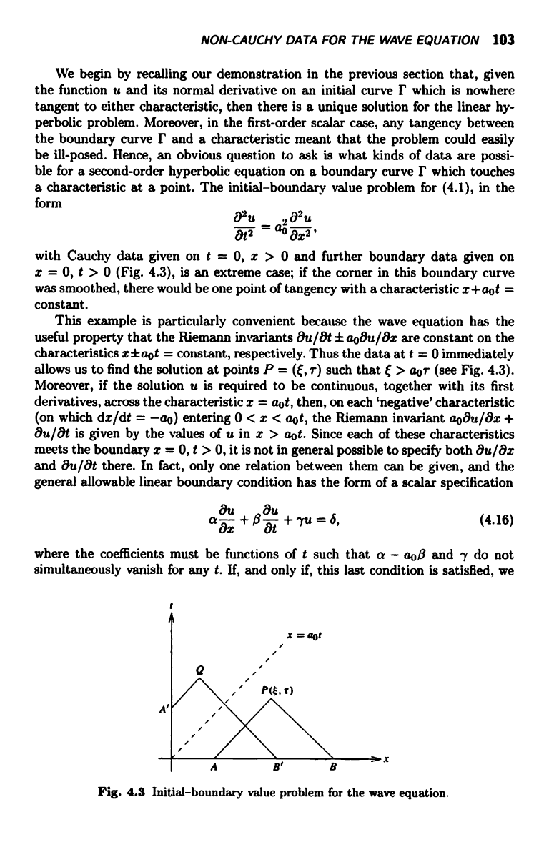
a characteristic at a point. The initial-boundary value problem for (4.1), in the

form

02u

202u

8t2 = %8x2,

with Cauchy data given on t = 0, x > 0 and further boundary data given on

x = 0, t > 0 (Fig. 4.3), is an extreme case; if the corner in this boundary curve

was smoothed, there would be one point of tangency with a characteristic x+aot =

constant.

This example is particularly convenient because the wave equation has the

useful property that the Riemann invariants Ou/8t±aoOu/8x are constant on the

characteristics x tact = constant, respectively. Thus the data at t = 0 immediately

allows us to find the solution at points P = (t;, r) such that t > aor (see Fig. 4.3).

Moreover, if the solution u is required to be continuous, together with its first

derivatives, across the characteristic x = aot, then, on each `negative' characteristic

(on which dx/dt = -ao) entering 0 < x < aot, the Riemann invariant aoOu/8x +

8u/8t is given by the values of u in x > aot. Since each of these characteristics

meets the boundary x = 0, t > 0, it is not in general possible to specify both 8u/8x

and &u/8t there. In fact, only one relation between them can be given, and the

general allowable linear boundary condition has the form of a scalar specification

asx+Q +ryu=6,

(4.16)

where the coefficients must be functions of t such that a - ao,5 and ry do not

simultaneously vanish for any t. If, and only if, this last condition is satisfied, we

Fig. 4.3 Initial-boundary value problem for the wave equation.

104 HYPERBOLIC EQUATIONS

(a)

(b)

Fig. 4.4 Space- and time-like boundaries.

can determine Ou/8x and Ou/8t on x = 0, t > 0, and hence obtain the solution at

the point Q in Fig. 4.3, from the R.iemann invariants along QA' and QB'. Of course,

the solution thus constructed usually has discontinuous second derivatives across

the characteristic x = aot. One way by which we could avoid such discontinuities

would be to `relax' the Cauchy data on x = 0. Indeed, if only u or Ou/8n was

prescribed on x = 0 for all t and on t = 0 for all x, we could find a solution as

smooth as the data, the Goursat problem of §3.5 being an example of this.

The discussion above illustrates the fact that if a boundary curve touches a

characteristic then Cauchy data can only be given on one side of the point of

tangency. The problem is, however, more or less symmetric in x and t so that it

is apparently immaterial on which side the Cauchy data is posed; in our example

this data could have been given on x = 0, t > 0 with only one condition on t = 0,

x > 0. However, in this case the characteristics of slope -ao would be propagating

the information Ou/Ot +aoOu/Ox = constant backwards in time, and such a model

may be said to violate causality. Thus, if we associate with the characteristics

a direction corresponding to time increasing, we are led to a characterisation of

well-posed initial-boundary value problems. For such problems Cauchy data is

prescribed on a curve whose slope dx/dt is always greater than ao in modulus,

and a single condition such as (4.16) is prescribed on a curve or curves whose

slope is always less than ao in modulus.

Although with just one space variable there is no mathematical reason for intro-

ducing causality, the concept of a time-like direction can sometimes be introduced

on physical grounds for other second-order hyperbolic equations. The discussion

above shows that we need a time-like variable t and a space-like variable x, and

two families of characteristics along each member of which a direction of increasing

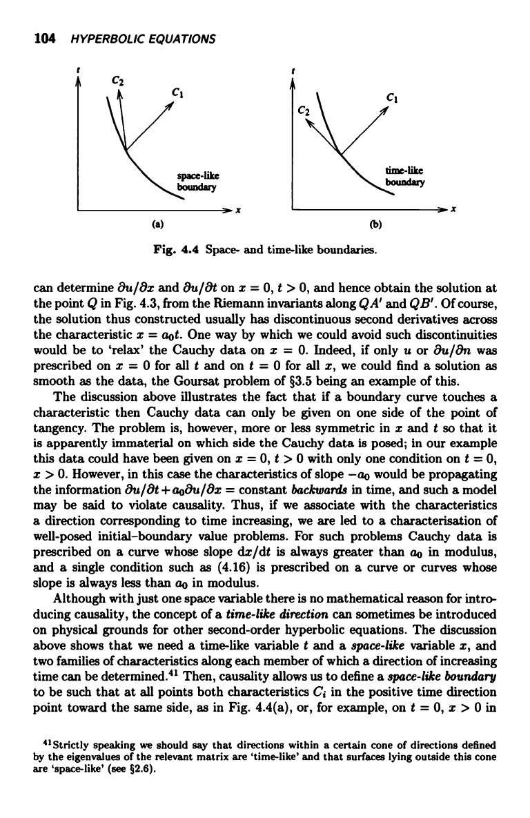
time can be determined."' Then, causality allows us to define a space-like boundary

to be such that at all points both characteristics C, in the positive time direction

point toward the same side, as in Fig. 4.4(a), or, for example, on t = 0, x > 0 in

41 Strictly speaking we should say that directions within a certain cone of directions defined

by the eigenvalues of the relevant matrix are 'time-like' and that surfaces lying outside this cone

are 'space-like' (see §2.6).

NON-CAUCHY DATA FOR THE WAVE EQUATION 105

Fig. 4.3. Likewise, a time-like boundary separates the characteristics in the positive

time direction, as in Fig. 4.4(b), or, for example, on z = 0, t > 0 in Fig. 4.3. We

need Cauchy data, involving two boundary conditions, on a space-like boundary

but only one condition is permissible on a time-like boundary, and, as in (4.16),

this condition must not contradict the information propagating along one of the

families of characteristics emanating from the Cauchy data.

*4.3.1

Strongly discontinuous boundary data

When the boundary data for a hyperbolic equation is not smooth, we may need

to generalise our idea of what constitutes a solution. In §2.5, we introduced weak

solutions for a first-order quasilinear hyperbolic system, and we now work through

these ideas for the simpler case of the wave equation

02u _

202u

ate

°`° e.r2

If the first derivatives of u are discontinuous at just one point of t = 0, say x = 0,

then the R.iemann function representation defines a solution which has continuous

derivatives except on x = fast. Following the ideas of weak solutions discussed

in §1.7 for scalar first-order equations, we say that a weak solution is a function u

which satisfies the identity

r- aoa

dxdt =

(0u

u4)

dx,

(4.17)

L0(

8t 8t

f=0

where (i is a twice-differentiable test function which vanishes suitably rapidly as

z -+ ±oo and t -+ oo. If u is twice differentiable, integration of (4.17) by parts

easily shows that it satisfies the wave equation everywhere in t > 0. However, we

emphasise that (4.17) is a mathematical statement that has no physical foundation

in any conservation law such as (1.24).

If, on the other hand, u is continuous but Vu is discontinuous across a `shock'

curve C, we know that [Ou/8x] dx + [Ou/8t] dt = 0 across C and,42 using an

argument similar to that used in obtaining the Rankine-Hugoniot condition (1.27),

we find

[fix ]

dt +

['u] dz

= 0,

(a2

for any test function t', so that l

[]dt+[8t]dx

=0. (4.18)

Thus, as expected, C is a characteristic through x = t = 0 with slope dx/dt = fao;

across C, ao[Ou/Ox] ± [Ou/8t] = 0 and we obtain the jump conditions necessary

to define the solution uniquely in -aot < x < aot. For the wave equation, these

42 We use the notation [

] in the same sense as in Chapter 1, to denote the jump from one side

of the shock to the other.

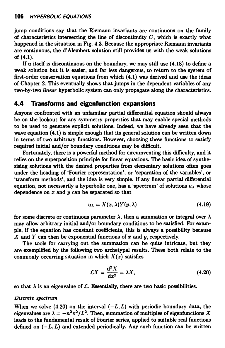
106 HYPERBOLIC EQUATIONS

jump conditions say that the Riemann invariants are continuous on the family

of characteristics intersecting the line of discontinuity C, which is exactly what

happened in the situation in Fig. 4.3. Because the appropriate Riemann invariants

are continuous, the d'Alembert solution still provides us with the weak solutions

of (4.1).

If u itself is discontinuous on the boundary, we may still use (4.18) to define a

weak solution but it is easier, and far less dangerous, to return to the system of

first-order conservation equations from which (4.1) was derived and use the ideas

of Chapter 2. This eventually shows that jumps in the dependent variables of any

two-by-two linear hyperbolic system can only propagate along the characteristics.

4.4 Transforms and eigenfunction expansions

Anyone confronted with an unfamiliar partial differential equation should always

be on the lookout for any symmetry properties that may enable special methods

to be used to generate explicit solutions. Indeed, we have already seen that the

wave equation (4.1) is simple enough that its general solution can be written down

in terms of two arbitrary functions. However, choosing these functions to satisfy

required initial and/or boundary conditions may be difficult.

Fortunately, there is a powerful method for circumventing this difficulty, and it

relies on the superposition principle for linear equations. The basic idea of synthe-

sising solutions with the desired properties from elementary solutions often goes

under the heading of 'Fourier representation', or `separation of the variables', or

'transform methods', and the idea is very simple. If any linear partial differential

equation, not necessarily a hyperbolic one, has a 'spectrum' of solutions ua whose

dependence on z and y can be separated so that

ua = X (x, A)Y(y, \)

(4.19)

for some discrete or continuous parameter \, then a summation or integral over A

may allow arbitrary initial and/or boundary conditions to be satisfied. For exam-

ple, if the equation has constant coefficients, this is always a possibility because

X and Y can then be exponential functions of x and y, respectively.

The tools for carrying out the summation can be quite intricate, but they

are exemplified by the following two archetypal results. These both relate to the

commonly occurring situation in which X (x) satisfies

LX = dxa = \X, (4.20)

so that A is an eigenvalue of L. Essentially, there are two basic possibilities.

Discrete spectrum

When we solve (4.20) on the interval (-L, L) with periodic boundary data, the

eigenvalues are A = -n2ir2/L2. Then, summation of multiples of eigenfunctions X

leads to the fundamental result of Fourier series, applied to suitable real functions

defined on (-L, L) and extended periodically. Any such function can be written

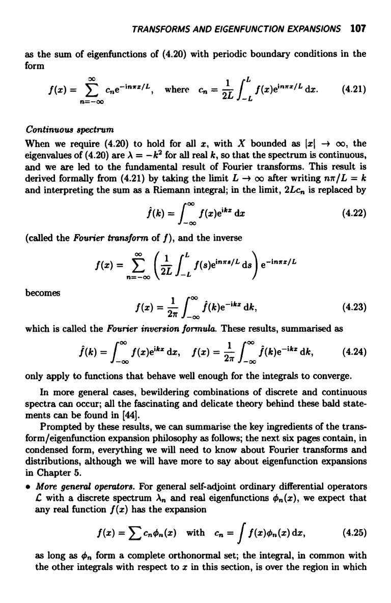
TRANSFORMS AND EIGENFUNCTION EXPANSIONS 107

as the sum of eigenfunctions of (4.20) with periodic boundary conditions in the

form

1 L

f (x) _

where

Cn =

f (x)cin,rz/L dx.

(4.21)

n=_oo

Continuous spectrum

When we require (4.20) to hold for all x, with X bounded as lxi -4 oo, the

eigenvalues of (4.20) are A = -k2 for all real k, so that the spectrum is continuous,

and we are led to the fundamental result of Fourier transforms. This result is

derived formally from (4.21) by taking the limit L -+ oo after writing nn/L = k

and interpreting the sum as a Riemann integral; in the limit, 2Lcn is replaced by

j (k)

= I

f (x)eikz dx

l 00

(called the Fourier transform of f), and the inverse

becomes

f (x) =

I f

(k)e-ikx dk,

(4.23)

which is called the Fourier inversion formula. Thesef results, summarised as

1 00

(k)e-!kx dk,

(4.24)

j (k)

(x)eikz dx,

f (x) = 2-

_00

only apply to functions that behave well enough for the integrals to converge.

In more general cases, bewildering combinations of discrete and continuous

spectra can occur; all the fascinating and delicate theory behind these bald state-

ments can be found in [44].

Prompted by these results, we can summarise the key ingredients of the trans-

form/eigenfunction expansion philosophy as follows; the next six pages contain, in

condensed form, everything we will need to know about Fourier transforms and

distributions, although we will have more to say about eigenfunction expansions

in Chapter 5.

More general operators. For general self-adjoint ordinary differential operators

C with a discrete spectrum An and real eigenfunctions qn(x), we expect that

any real function f (x) has the expansion

ff(x)4(x)dx,

f (x) =

C(x) with

Cn =

(4.25)

as long as On form a complete orthonormal set; the integral, in common with

the other integrals with respect to x in this section, is over the region in which

(4.22)

f(x) 1

f L f(s)einne/L d8)

C_inaz/L

n-j I\2L J_L