Moran M.J., Shapiro H.N. Fundamentals of Engineering Thermodynamics

Подождите немного. Документ загружается.

206

ENGINEERING CONTEXT Up to this point, our study of the sec-

ond law has been concerned primarily with what it says about systems undergoing

thermodynamic cycles. In this chapter means are introduced for analyzing systems from

the second law perspective as they undergo processes that are not necessarily cycles.

The property entropy plays a prominent part in these considerations. The objective of the

present chapter is to introduce entropy and show its use for thermodynamic analysis.

The word energy is so much a part of the language that you were undoubtedly familiar

with the term before encountering it in early science courses. This familiarity probably

facilitated the study of energy in these courses and in the current course in engineering

thermodynamics. In the present chapter you will see that the analysis of systems from a

second law perspective is conveniently accomplished in terms of the property entropy.

Energy and entropy are both abstract concepts. However, unlike energy, the word entropy is

seldom heard in everyday conversation, and you may never have dealt with it quantitatively

before. Energy and entropy play important roles in the remaining chapters of this book.

Using Entropy

chapter objective 



6.1 Introducing Entropy

Corollaries of the second law are developed in Chap. 5 for systems undergoing cycles while

communicating thermally with two reservoirs, a hot reservoir and a cold reservoir. In the

present section a corollary of the second law known as the Clausius inequality is introduced

that is applicable to any cycle without regard for the body, or bodies, from which the cycle

receives energy by heat transfer or to which the cycle rejects energy by heat transfer. The

Clausius inequality provides the basis for introducing two ideas instrumental for analyses of

both closed systems and control volumes from a second law perspective: the property entropy

(Sec. 6.2) and the entropy balance (Secs. 6.5 and 6.6).

The Clausius inequality states that for any thermodynamic cycle

(6.1)

where Q represents the heat transfer at a part of the system boundary during a portion of the

cycle, and T is the absolute temperature at that part of the boundary. The subscript “b” serves

as a reminder that the integrand is evaluated at the boundary of the system executing the cycle.

The symbol indicates that the integral is to be performed over all parts of the boundary and





 0

Clausius inequality

6.1 Introducing Entropy 207

over the entire cycle. The equality and inequality have the same interpretation as in the

Kelvin–Planck statement: the equality applies when there are no internal irreversibilities as

the system executes the cycle, and the inequality applies when internal irreversibilities are

present. The Clausius inequality can be demonstrated using the Kelvin–Planck statement of

the second law (see box).

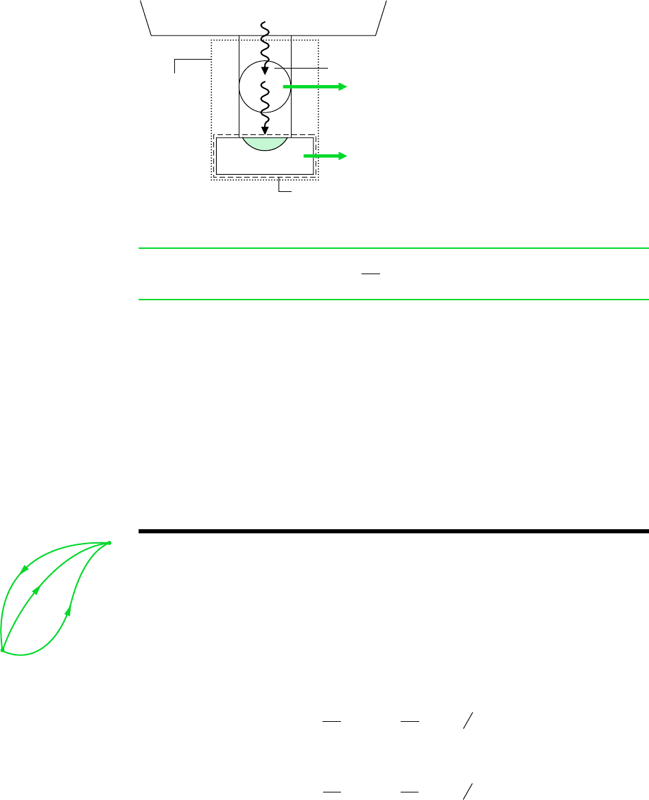
DEVELOPING THE CLAUSIUS INEQUALITY

The Clausius inequality can be demonstrated using the arrangement of Fig. 6.1. A sys-

tem receives energy Q at a location on its boundary where the absolute temperature

is T while the system develops work W. In keeping with our sign convention for heat

transfer, the phrase receives energy Q includes the possibility of heat transfer from

the system. The energy Q is received from (or absorbed by) a thermal reservoir at

res

. To ensure that no irreversibility is introduced as a result of heat transfer between

the reservoir and the system, let it be accomplished through an intermediary system

that undergoes a cycle without irreversibilities of any kind. The cycle receives energy

Q from the reservoir and supplies Q to the system while producing work W. From

the definition of the Kelvin scale (Eq. 5.6), we have the following relationship between

the heat transfers and temperatures:

(a)

As temperature may vary, a multiplicity of such reversible cycles may be required.

Consider next the combined system shown by the dotted line on Fig. 6.1. An en-

ergy balance for the combined system is

where W

is the total work of the combined system, the sum of W and W, and dE

denotes the change in energy of the combined system. Solving the energy balance for

W

and using Eq. (a) to eliminate Q from the resulting expression yields

Now, let the system undergo a single cycle while the intermediary system undergoes

one or more cycles. The total work of the combined system is

(b)

Since the reservoir temperature is constant, T

res

can be brought outside the integral. The

term involving the energy of the combined system vanishes because the energy change

for any cycle is zero. The combined system operates in a cycle because its parts exe-

cute cycles. Since the combined system undergoes a cycle and exchanges energy by

heat transfer with a single reservoir, Eq. 5.1 expressing the Kelvin–Planck statement

of the second law must be satisfied. Using this, Eq. (b) reduces to give Eq. 6.1, where

the equality applies when there are no irreversibilities within the system as it executes

the cycle and the inequality applies when internal irreversibilities are present. This in-

terpretation actually refers to the combination of system plus intermediary cycle. How-

ever, the intermediary cycle is regarded as free of irreversibilities, so the only possible

site of irreversibilities is the system alone.





res





 T

res



 T

res

 dE

 dQ¿  dW

dQ¿

res

 a

Equation 6.1 can be expressed equivalently as

(6.2)

where 

cycle

can be viewed as representing the “strength” of the inequality. The value of 

cycle

is positive when internal irreversibilities are present, zero when no internal irreversibilities

are present, and can never be negative. In summary, the nature of a cycle executed by a sys-

tem is indicated by the value for 

cycle

as follows:

Accordingly, 

cycle

is a measure of the effect of the irreversibilities present within the system

executing the cycle. This point is developed further in Sec. 6.5, where 

cycle

is identified as

the entropy produced (or generated) by internal irreversibilities during the cycle.

cycle

6 0

impossible

cycle

7 0

irreversibilities present within the system

cycle

 0

no irreversibilities present within the system



s

cycle

208 Chapter 6 Using Entropy



6.2 Defining Entropy Change

A quantity is a property if, and only if, its change in value between two states is independ-

ent of the process (Sec. 1.3). This aspect of the property concept is used in the present sec-

tion together with Eq. 6.2 to introduce entropy.

Two cycles executed by a closed system are represented in Fig. 6.2. One cycle consists

of an internally reversible process A from state 1 to state 2, followed by internally reversible

process C from state 2 to state 1. The other cycle consists of an internally reversible process

B from state 1 to state 2, followed by the same process C from state 2 to state 1 as in the

first cycle. For the first cycle, Eq. 6.2 takes the form

(6.3a)

and for the second cycle

(6.3b)

In writing Eqs. 6.3, the term 

cycle

has been set to zero since the cycles are composed of

internally reversible processes.



 a



s

cycle



 a



s

cycle

Reservoir at T

res

Intermediary

cycle

System boundary

δW´

δQ´

δQ

δW

Combined

system

boundary

System

 Figure 6.1 Illustration used to develop the

Clausius inequality.

 Figure 6.2 Two in-

ternally reversible cycles.

6.3 Retrieving Entropy Data 209

When Eq. 6.3b is subtracted from Eq. 6.3a

This shows that the integral of QT is the same for both processes. Since A and B are ar-

bitrary, it follows that the integral of QT has the same value for any internally reversible

process between the two states. In other words, the value of the integral depends on the end

states only. It can be concluded, therefore, that the integral represents the change in some

property of the system.

Selecting the symbol S to denote this property, which is called entropy, its change is

given by

(6.4a)

where the subscript “int rev” is added as a reminder that the integration is carried out for

any internally reversible process linking the two states. Equation 6.4a is the definition of

entropy change. On a differential basis, the defining equation for entropy change takes

the form

(6.4b)

Entropy is an extensive property.

The SI unit for entropy is J/K. However, in this book it is convenient to work in terms

of kJ/K. Units in SI for specific entropy are kJ/kg K for s and kJ/kmol K for

Since entropy is a property, the change in entropy of a system in going from one state to

another is the same for all processes, both internally reversible and irreversible, between these

two states. Thus, Eq. 6.4a allows the determination of the change in entropy, and once it has

been evaluated, this is the magnitude of the entropy change for all processes of the system

between the two states. The evaluation of entropy change is discussed further in the next

section.

It should be clear that entropy is defined and evaluated in terms of a particular integral

for which no accompanying physical picture is given. We encountered this previously with

the property enthalpy. Enthalpy is introduced without physical motivation in Sec. 3.3.2. Then,

in Chap. 4, enthalpy is shown to be useful for thermodynamic analysis. As for the case of

enthalpy, to gain an appreciation for entropy you need to understand how it is used and what

it is used for.

dS  a

rev

int

 S

 a



rev

int



 a



6.3 Retrieving Entropy Data

In Chap. 3, we introduced means for retrieving property data, including tables, graphs, equa-

tions, and the software available with this text. The emphasis there is on evaluating the prop-

erties p, v, T, u, and h required for application of the conservation of mass and energy

principles. For application of the second law, entropy values are usually required. In this

section, means for retrieving entropy data are considered.

definition of entropy

change

units for entropy

 6.3.1 General Considerations

The defining equation for entropy change, Eq. 6.4a, serves as the basis for evaluating en-

tropy relative to a reference value at a reference state. Both the reference value and the ref-

erence state can be selected arbitrarily. The value of the entropy at any state y relative to the

value at the reference state x is obtained in principle from

(6.5)

where S

is the reference value for entropy at the specified reference state.

The use of entropy values determined relative to an arbitrary reference state is satisfac-

tory as long as they are used in calculations involving entropy differences, for then the ref-

erence value cancels. This approach suffices for applications where composition remains con-

stant. When chemical reactions occur, it is necessary to work in terms of absolute values of

entropy determined using the third law of thermodynamics (Chap. 13).

ENTROPY DATA FOR WATER AND REFRIGERANTS

Tables of thermodynamic data are introduced in Sec. 3.3 for water and several refrigerants

(Tables A-2 through A-18). Specific entropy is tabulated in the same way as considered there

for the properties v, u, and h, and entropy values are retrieved similarly.

VAPOR DATA. In the superheat regions of the tables for water and the refrigerants, specific

entropy is tabulated along with v, u, and h versus temperature and pressure.

 for example. . . consider two states of water. At state 1 the pressure is 3 MPa and the

temperature is 500C. At state 2, the pressure is 0.3 MPa and the specific entropy is the same

as at state 1, s

 s

. The object is to determine the temperature at state 2. Using T

and p

we find the specific entropy at state 1 from Table A-4 as s

 7.2338 kJkg K. State 2 is

fixed by the pressure, p

 0.3 MPa, and the specific entropy, s

 7.2338 kJkg K. Returing

to Table A-4 at 0.3 MPa and interpolating with s

between 160 and 200C results in

 183C. 

SATURATION DATA. For saturation states, the values of s

and s

are tabulated as a func-

tion of either saturation pressure or saturation temperature. The specific entropy of a two-

phase liquid–vapor mixture is calculated using the quality

(6.6)

These relations are identical in form to those for v, u, and h (Sec. 3.3).  for example. . .

let us determine the specific entropy of Refrigerant 134a at a state where the temperature

is 0C and the specific internal energy is 138.43 kJ/kg. Referring to Table A-10, we see that

the given value for u falls between u

and u

at 0C, so the system is a two-phase liquid–vapor

mixture. The quality of the mixture can be determined from the known specific internal

energy

Then with values from Table A-10



 10.5210.19702 10.5210.91902 0.5580 kJ/kg

s  11  x2s

 xs

x 

u  u

 u



138.43  49.79

227.06  49.79

 0.5

s  11  x2s

 xs

 s

 x1s

 s

 S

 a



rev

int

210 Chapter 6 Using Entropy



6.3 Retrieving Entropy Data 211

LIQUID DATA. Compressed liquid data are presented for water in Tables A-5. In these tables

s, v, u, and h are tabulated versus temperature and pressure as in the superheat tables, and

the tables are used similarly. In the absence of compressed liquid data, the value of the specific

entropy can be estimated in the same way as estimates for v and u are obtained for liquid

states (Sec. 3.3.6), by using the saturated liquid value at the given temperature

(6.7)

 for example. . .

suppose the value of specific entropy is required for water at 25 bar,

200C. The specific entropy is obtained directly from Table A-5 as s  2.3294 kJkg K. Using

the saturated liquid value for specific entropy at 200C from Table A-2, the specific entropy

is approximated with Eq. 6.7 as s  2.3309 kJkg K, which agrees closely with the previous

value. 

The specific entropy values for water and the refrigerants given in Tables A-2 through

A-18 are relative to the following reference states and values. For water, the entropy of

saturated liquid at 0.01C is set to zero. For the refrigerants, the entropy of the saturated liq-

uid at 40C is assigned a value of zero.

COMPUTER RETRIEVAL. The software available with this text, Interactive Thermodynam-

ics: IT, provides data for the substances considered in this section. Entropy data are retrieved

by simple call statements placed in the workspace of the program.  for example. . .

consider a two-phase liquid–vapor mixture of H

O at p  1 bar, v  0.8475 m

/kg. The fol-

lowing illustrates how specific entropy and quality x are obtained using IT

p = 1 // bar

v = 0.8475 // m

/kg

v = vsat_Px(“Water/Steam”,p,x)

s = ssat_Px(“Water/Steam”,p,x)

The software returns values of x  0.5 and s  4.331 kJ/kg K, which can be checked using

data from Table A-3. Note that quality x is implicit in the list of arguments in the expression

for specific volume, and it is not necessary to solve explicitly for x. As another example, con-

sider superheated ammonia vapor at p  1.5 bar, T  8C. Specific entropy is obtained from

IT as follows:

p = 1.5 // bar

T = 8 // C

s = s_PT(“Ammonia”,p,T)

The software returns s  5.981 kJ/kg K, which agrees closely with the value obtained by

interpolation in Table A-15. 

USING GRAPHICAL ENTROPY DATA

The use of property diagrams as an adjunct to problem solving is emphasized throughout

this book. When applying the second law, it is frequently helpful to locate states and plot

processes on diagrams having entropy as a coordinate. Two commonly used figures having

entropy as one of the coordinates are the temperature–entropy diagram and the enthalpy–

entropy diagram.

TEMPERATURE–ENTROPY DIAGRAM. The main features of a temperature–entropy

diagram are shown in Fig. 6.3. For detailed figures for water in SI, see Fig. A-7. Observe

s1T, p2 s

1T 2

METHODOLOGY

UPDATE

Note that IT does not

provide compressed liquid

data for any substance. IT

returns liquid entropy data

using the approximation of

Eq. 6.7. Similarly, Eqs. 3.11,

3.12, and 3.14 are used to

return liquid values for v,

u, and h, respectively.



T–s diagram

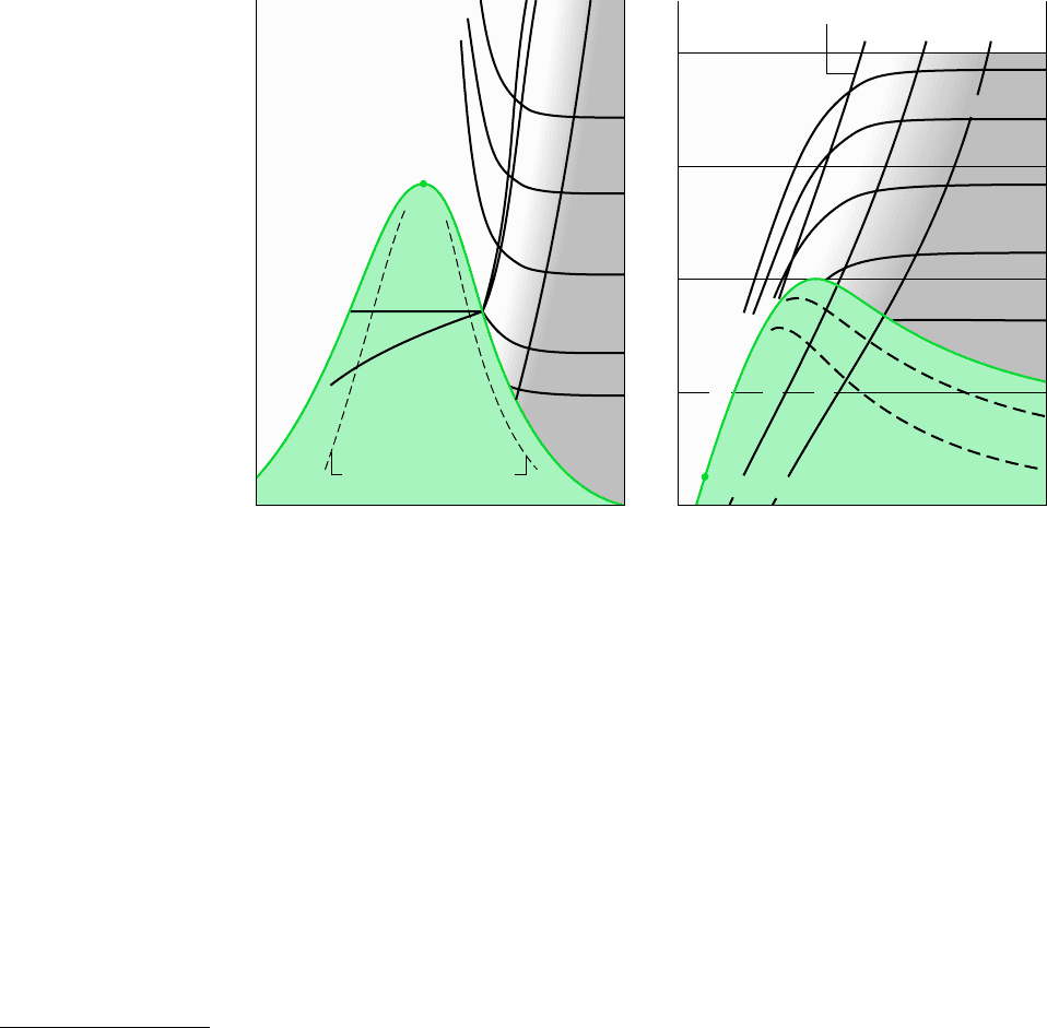
that lines of constant enthalpy are shown on these figures. Also note that in the super-

heated vapor region constant specific volume lines have a steeper slope than constant-

pressure lines. Lines of constant quality are shown in the two-phase liquid–vapor region.

On some figures, lines of constant quality are marked as percent moisture lines. The per-

cent moisture is defined as the ratio of the mass of liquid to the total mass.

In the superheated vapor region of the T–s diagram, constant specific enthalpy lines be-

come nearly horizontal as pressure is reduced. These states are shown as the shaded area on

Fig. 6.3. For states in this region of the diagram, the enthalpy is determined primarily by the

temperature: h(T, p)  h(T). This is the region of the diagram where the ideal gas model

provides a reasonable approximation. For superheated vapor states outside the shaded area,

both temperature and pressure are required to evaluate enthalpy, and the ideal gas model is

not suitable.

ENTHALPY–ENTROPY DIAGRAM. The essential features of an enthalpy–entropy diagram,

commonly known as a Mollier diagram, are shown in Fig. 6.4. For detailed figures for water

in SI, see Figs. A-8. Note the location of the critical point and the appearance of lines of

constant temperature and constant pressure. Lines of constant quality are shown in the two-

phase liquid–vapor region (some figures give lines of constant percent moisture). The figure

is intended for evaluating properties at superheated vapor states and for two-phase liquid–

vapor mixtures. Liquid data are seldom shown. In the superheated vapor region, constant-

temperature lines become nearly horizontal as pressure is reduced. These states are shown,

approximately, as the shaded area on Fig. 6.4. This area corresponds to the shaded area on

the temperature–entropy diagram of Fig. 6.3, where the ideal gas model provides a reasonable

approximation.

 for example. . . to illustrate the use of the Mollier diagram in SI units, consider

two states of water. At state 1, T

 240C, p

 0.10 MPa. The specific enthalpy and

212 Chapter 6 Using Entropy

Critical point

p = constant

v = constant

x = 0.2 x = 0.9

= constant

v = constant

p = constant

T = constant

p = constant

Critical point

 Figure 6.3 Temperature–entropy diagram.

 Figure 6.4 Enthalpy–entropy diagram.

Mollier diagram

6.3 Retrieving Entropy Data 213

first T dS equation

second T dS equation

quality are required at state 2, where p

 0.01 MPa and s

 s

. Turning to Fig. A-8, state 1

is located in the superheated vapor region. Dropping a vertical line into the two-phase

liquid–vapor region, state 2 is located. The quality and specific enthalpy at state 2 read

from the figure agree closely with values obtained using Tables A-3 and A-4: x

 0.98 and

 2537 kJ/kg. 

USING THE T dS EQUATIONS

Although the change in entropy between two states can be determined in principle by using

Eq. 6.4a, such evaluations are generally conducted using the T dS equations developed in

this section. The T dS equations allow entropy changes to be evaluated from other more read-

ily determined property data. The use of the T dS equations to evaluate entropy changes for

ideal gases is illustrated in Sec. 6.3.2 and for incompressible substances in Sec. 6.3.3. The

importance of the T dS equations is greater than their role in assigning entropy values, how-

ever. In Chap. 11 they are used as a point of departure for deriving many important property

relations for pure, simple compressible systems, including means for constructing the prop-

erty tables giving u, h, and s.

The T dS equations are developed by considering a pure, simple compressible system un-

dergoing an internally reversible process. In the absence of overall system motion and the

effects of gravity, an energy balance in differential form is

(6.8)

By definition of simple compressible system (Sec. 3.1), the work is

(6.9a)

On rearrangement of Eq. 6.4b, the heat transfer is

(6.9b)

Substituting Eqs. 6.9 into Eq. 6.8, the first T dS equation results

(6.10)

The second T dS equation is obtained from Eq. 6.10 using H  U  pV. Forming the

differential

On rearrangement

Substituting this into Eq. 6.10 gives the second T dS equation

(6.11)

The T dS equations can be written on a unit mass basis as

(6.12a)

(6.12b)

T ds  dh  v dp

T ds  du  p dv

T dS  dH  V dp

dU  p dV  dH  V dp

dH  dU  d1

pV2 dU  p dV  V dp

dS  dU  p dV

1dQ2

int

rev

 T

1dW2

int

rev

 p

1dQ2

int

rev

 dU  1dW2

int

rev

or on a per mole basis as

(6.13a)

(6.13b)

Although the T dS equations are derived by considering an internally reversible process,

an entropy change obtained by integrating these equations is the change for any process, re-

versible or irreversible, between two equilibrium states of a system. Because entropy is a

property, the change in entropy between two states is independent of the details of the process

linking the states.

To show the use of the T dS equations, consider a change in phase from saturated liquid

to saturated vapor at constant temperature and pressure. Since pressure is constant, Eq. 6.12b

reduces to give

Then, because temperature is also constant during the phase change

(6.14)

This relationship shows how s

 s

is calculated for tabulation in property tables.

 for example. . . consider Refrigerant 134a at 0C. From Table A-10, h

 h



197.21 kJ/kg, so with Eq. 6.14

which is the value calculated using s

and s

from the table. 

 6.3.2 Entropy Change of an Ideal Gas

In this section the T dS equations are used to evaluate the entropy change between two states

of an ideal gas. It is convenient to begin with Eqs. 6.12 expressed as

(6.15)

(6.16)

For an ideal gas, du  c

(T) dT, dh  c

(T) dT, and pv  RT. With these relations,

Eqs. 6.15 and 6.16 become, respectively

(6.17)

Since R is a constant, the last terms of Eqs. 6.17 can be integrated directly. However, because

and c

are functions of temperature for ideal gases, it is necessary to have information about

ds  c

1T 2

 R

and

ds  c

1T 2

 R

ds 



ds 



 s



197.21

kJ/kg

273.15 K

 0.7220

 s



 h

ds 

T d s  d h  v dp

T d s  d u  p d v

214 Chapter 6 Using Entropy

6.3 Retrieving Entropy Data 215

the functional relationships before the integration of the first term in these equations can be

performed. Since the two specific heats are related by

(3.44)

where R is the gas constant, knowledge of either specific heat function suffices.

On integration, Eqs. 6.17 give, respectively

(6.18)

(6.19)

USING IDEAL GAS TABLES. As for internal energy and enthalpy changes, the evaluation

of entropy changes for ideal gases can be reduced to a convenient tabular approach. To in-

troduce this, we begin by selecting a reference state and reference value: The value of the spe-

cific entropy is set to zero at the state where the temperature is 0 K and the pressure is 1 at-

mosphere. Then, using Eq. 6.19, the specific entropy at a state where the temperature is T and

the pressure is 1 atm is determined relative to this reference state and reference value as

(6.20)

The symbol s(T ) denotes the specific entropy at temperature T and a pressure of 1 atm.

Because s depends only on temperature, it can be tabulated versus temperature, like

h and u. For air as an ideal gas, s with units of is given in Tables A-22.Values

of for several other common gases are given in Tables A-23 with units of .

Since the integral of Eq. 6.19 can be expressed in terms of s

it follows that Eq. 6.19 can be written as

(6.21a)

or on a per mole basis as

(6.21b)

Using Eqs. 6.21 and the tabulated values for s or as appropriate, entropy changes

can be determined that account explicitly for the variation of specific heat with temperature.

 for example. . . let us evaluate the change in specific entropy, in kJkg K, of air

modeled as an ideal gas from a state where T

 300 K and p

 1 bar to a state where

°,

, p

2 s1T

, p

2 s °1T

2 s °1T

2 R ln

s1T

, p

2 s1T

, p

2 s°1T

2 s°1T

2 R ln

 s°1T

2 s°1T











kJ/kmol

Ks °

kJ/kg

s°1T 2



1T 2

s1T

, p

2 s1T

, p

2



1T 2

 R ln

s1T

2 s1T

, v

2



1T 2

 R ln

1T 2 c

1T 2 R

