Moller K.D. Optics. Learning by Computing, with Examples Using Mathcad, Matlab, Mathematica, and Maple
Подождите немного. Документ загружается.

7.6. CONFOCAL CAVITY, GAUSSIAN BEAM, AND MODES 309
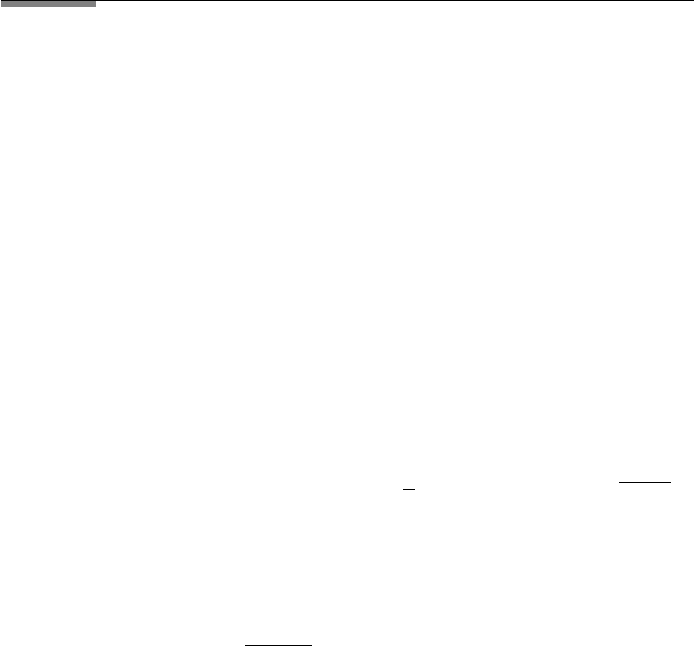
In FileFig 7.12a we show graphs of the first four modes from (0,0) to (1,1). In
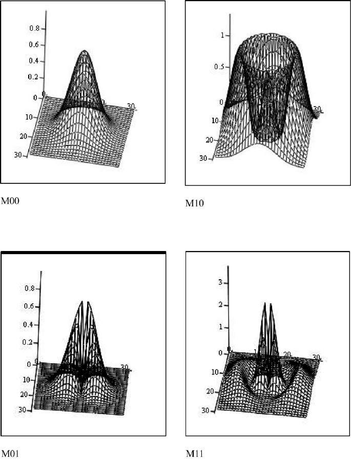
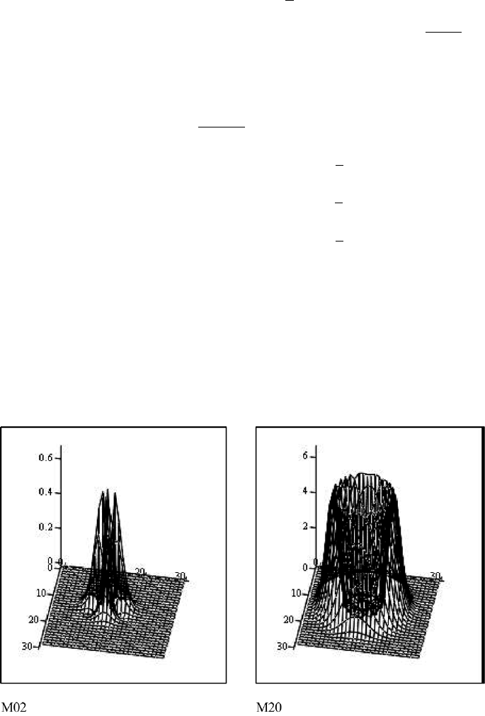
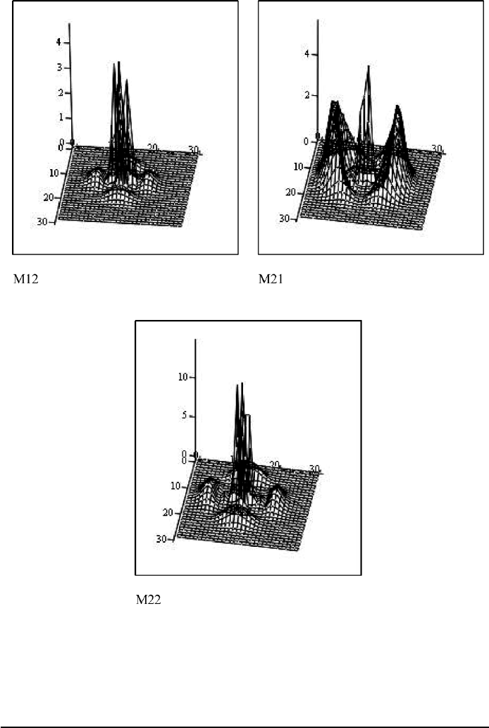
FileFig 7.12b we show graphs of the next five modes from (1,2) to (2,2). Contour
plots were chosen for better reference to Figure 7.21, and identification of the
zero-intensity lines and mode numbers.
FileFig 7.12 (L12MOCY1to4S)(L12MOCY5to9S)
Modes for confocal cavity and circular mirrors. Contour plots of generalized
Laguerre polynomial for indices l and p equal 0, 1, and 2. Scaling factor is X.
L12MOCY1to4S
Cylindrical Coordinates for Circular Mirrors in Confocal Resonator
Field distribution as contour plot for graph 00, 10, 01, and 11. The L(l, p)
functions are written out for 00 to 22. The constant in the exponential is X:
i : 0 ...N j : 0 ...N N 40
x
i
: (−2) + .10001 · iy
j
: (−2) + .10001 · j
R(x, y): (x)
2
+ (y)
2
β(x,y):
a tan
x
y
2
q(x,y):
e
−(R(x,y))
x
.
Constant X : X ≡ 3. The L’s are given below.
u(x,y): 4 ·
R(x, y)
X
g(x, y): cos(0 · β(x,y))
L00(x,y): 1 L01(x,y): 1 − u(x, y)
L10(x,y): 1 L11(x,y): 2 −u(x, y)
M00
i,j
: (cos(0 · β(x
i
,y
j
)) · q(x
i
,y
j
) · L00(x
i
,y
j
))
2
M10
i,j
: (cos(0 · β(x
i
,y
j
)) · q(x
i
,y
j
) · L01(x
i
,y
j
))
2
.
310 7. BLACKBODY RADIATION, ATOMIC EMISSION, AND LASERS
M01
i,j
: (cos(1 · β(x
i
,y
j
)) · q(x
i
,y
j
) · L10(x
i
,y
j
))
2
M11
i,j
: (cos(1 · β(x
i
,y
j
)) · q(x
i
,y
j
) · L11(x
i
,y
j
))
2
.
L12MOCY5to9S
Cylindrical Coordinates for Circular Mirrors in Confocal Resonator
Field distribution as contour plot for graph 02 to 20. The L(l,p) functions are
written out for 00 to 22. The constant in the exponential is X:
i : 0 ...N j : 0 ...N N 40
7.6. CONFOCAL CAVITY, GAUSSIAN BEAM, AND MODES 311
x
i
: (−2) + .10001 · iy
j
: (−2) + .10001 · j
R(x, y): (x)
2
+ (y)
2
β(x,y):
a tan
x
y
2
q(x,y):
e
−(R(x,y))
x
.
Constant X : X ≡ 2. There h stands for l and p runs from 0 to 2.
Lh2(x,y): [1/2(h + 1)(h + 2) −(h + 2)u(x, y)] + (1/2)u(x,y)
2
u(x,Y): 4 ·
R(x, y)
X
g(x, y): cos(0 · β(x,y))
L02(x,y): 1 − 2 ·u(x, y) +
1
2
· u(x,y)
2
L22
(
x,y): 6 − 4 ·u(x, y) +
1
2
· u(x,y)
2
L12(x,y): 3 − 3 · u(x, y) +
1
2
· u(x,y)
2
L21(x,y): 3 − u(x, y)
L20(x,y): 1.
M02
i,j
: (cos(2 ·β(x
i
,y
j
)) · q(x
i
,y
j
) · L20(x
i
,y
j
))
2
M20
i,j
: (cos(0 · β(x
i
,y
j
)) · q(x
i
,y
j
) · L02(x
i
,y
j
))
2
.
312 7. BLACKBODY RADIATION, ATOMIC EMISSION, AND LASERS
M12
i,j
: (cos(2 ·β(x
i
,y
j
)) · q(x
i
,y
j
) · L21(x
i
,y
j
))
2
M21
i,j
: (cos(1 · β(x
i
,y
j
)) · q(x
i
,y
j
) · L12(x
i
,y
j
))
2
.
M22
i,j
: (cos(2 ·β(x
i
,y
j
)) · q(x
i
,y
j
) · L22(x
i
,y
j
))
2
.
Application 7.12.
1. Compare with Figure 7.21 and the number of zero intensity lines with the
mode numbers.
2. Convert surface to contour plots and try to identify the modes.
7.6. CONFOCAL CAVITY, GAUSSIAN BEAM, AND MODES 313
PL1. Rayleigh-Jeans Law and Planck’s Law (see p. 271).
PL2. Graph of Black Body Radiation depending on Wavelength and Fre-
quency.(see p. 275–277).
PL3. Lorentzian Line Shape with angular Resonance frequency ω
o
and
Lifetime τ (see p. 284).
PL4. Calculation of (N
2
− N
1
)/N
o
(see p. 292).
PL5. Paraxial Wave Equation (see p. 294).
PL6. Calculation of w
2
(z) and R(z) for Confocal Cavity (see p. 296).
PL7. Modes for Confocal Cavity and rectangular Mirrors (see p. 300).
PL8. Modes for Confocal Cavity and circular Mirrors (see p. 305).

8
8
CHAPTER
Optical
Constants
8.1 INTRODUCTION
In the chapters on geometrical optics, interference, and electromagnetic theory
we have sometimes used the refractive index n c/v. When light enters a
dielectric medium, it interacts with the atoms and changes its speed from c in
vacuum to v in the medium. The medium is called isotropic when the speed of
light is the same in all directions. The refractive index may be obtained from
the real part of the dielectric constant in Maxwell’s equations. In the case where
there are losses in the medium, light will be absorbed, and one uses the complex
dielectric constant in Maxwell’s equations.
In this chapter we first look at the dielectric constants in Maxwell’s equations
and then use a simple model for the analytical representation. As a result we
get the index of refraction depending on the frequency of the light and model
parameters. The model we use is a damped forced oscillator. The incident light
drives these oscillators, representing the material, and loses some of its intensity.
The losses of the electromagnetic wave are described by a complex refractive
index (n − iK). In books on solid state physics the complex refractive index is
often called n + iκ (and not n − iK). We have to relate n and K or κ, called
optical constants, to the parameters of our model.
315

316 8. OPTICAL CONSTANTS
8.2 OPTICAL CONSTANTS OF DIELECTRICS
8.2.1 The Wave Equation, Electrical Polarizability, and
Refractive Index
We write Maxwell’s equations for an isotropic and nonmagnetic material without
free charges, which means we assume ∇·P 0 and ρ 0 and have
∇×E −∂B/∂t
c
2
∇×B ∂E/∂t +j/ε
0
(8.1)
∇·E 0
∇·B 0,
where E is the electrical field vector, B the magnetic field vector, j the current
density vector ρ the charge density, and ε
0
8.854×10
−12
F/m, the permittivity
of vacuum. We now study the effect of an outside electrical field on the bound
charges in an isotropic material. The outside electrical field is assumed to be a
harmonic wave and will act on the bound charges and make them vibrate. For
the current density N of such vibrating charges we have
j Nev, (8.2)
where N is the number of charges per unit volume, e the charge of the electron,
and v the velocity vector. Since we assume an isotropic medium, we only have to
take into account one direction of vibration, which we call y, and one direction
of motion, which we call x. With v dx/dt we have
j
y
Ne dx/dt. (8.3)
The induced dipoles are ex, and P N (ex) is called the polarization. The
current density is then
j
y
dP
y
/dt. (8.4)
The wave equation for vibration in the y direction and propagation in the x
direction is
∂
2
E
y
/∂x
2
− (1/c
2
)∂
2
E
y
/∂t
2
[1/(ε
0
c
2
)]∂
2
P
y
/∂t
2
, (8.5)
where the right side of Eq. (8.5) is called the source term.
In the first approximation, we set P
y
proportional to the incident electrical
field and write
P
y
ε
0
NαE
y
, (8.6)
where α is the atomic polarizability, a constant characteristic for the material.
We introduce into the wave equation a trial solution E
y
A cos(kx − ωt), and
get
−k
2
E
y
+ (1/c
2
)ω
2
E
y
(1/ε
0
c
2
)(−ω
2
αE
y
) (8.7)
8.2. OPTICAL CONSTANTS OF DIELECTRICS 317
or
k
2
(ω
2
/c
2
)(1 + Nα). (8.8)
We associate the velocity v with the the phase velocity ω/k in the medium and
obtain for n
n
2
c
2
/v
2
c
2
k
2
/ω
2
(1 + Nα). (8.9)
We have obtained a relation between the optical constant n and the material
constant α, the atomic polarizability.
8.2.2 Oscillator Model and the Wave Equation
8.2.2.1 Less Dense Medium
To study the dependence of the refractive index on frequencies and losses, we
relate the refractive index to the parameters of an oscillator model.
The polarization vector P of the medium is defined as the number of electrical
dipoles per unit volume. The induced electrical dipole moment is eE
y
, which
we now call (eu), where u is the displacement of an electron in an atom. The
number of dipoles per unit volume is N and we consider only one component of
vibration y and have
P Neu. (8.10)
We describe the displacement u of the charges by the vibrations of a damped
oscillator,
md
2
u/dt
2
+ mγ du/dt + mω
2
0
u 0, (8.11)
where u is the displacement of the charge from its equilibrium position, m is
the mass, f the force, and γ the damping constant. The frequency without the
damping term is ω
12
0
f/m, and the resonance frequency for the damped oscil-
lator is ω
0
ω
0
. The electromagnetic wave of the light drives these oscillators.
The forced damped oscillator equation is
md
2
u/dt
2
+ mγ du/dt + mω
2
0
u eE
o
e
−iωt
. (8.12)
We introduce the trial solution Ae
−iωt
and obtain
u(t) [eE(t)/m]/[(ω
2
0
− ω
2
) − iγω], (8.13)
where E(t) E
0
e
−iωt
. The driving electromagnetic wave produces polarization
P (t) Neu(t) [Ne
2
ε
o
E(t)]/[mε
o
(ω
2
0
− ω
2
− iγω)] χ
∗
ε
0
E(t), (8.14)
where ε
0
is the permittivity of free space. As a result of the imaginary damping
term in u(t) one has a complex susceptibility χ , indicated by a star. In Eq. (8.14)
we have related the polarization P (t) and the electrical susceptibility χ to the
parameters of our model and the electrical field E(t) of the light.

318 8. OPTICAL CONSTANTS
From the wave equation, we have another expression of P (t) (see Eq. (8.6))
and introducing P (t) ε
0
NαE(t) into Eq. (8.14) we get
α (1/N)ω
2
p
/(ω
2
0
− ω
2
− iγω), (8.15)
where α is the atomic polarizability and ω
2
p
Ne
2
/mε
0
the plasma frequency.
One should not confuse this with ω
2
0
, the square of the angular frequency of the
oscillator model, representing the dielectric.We have obtained a relation between
the material constant of the atomic polarizability α and the parameters of our
oscillator model. For the square of the refractive index, (see eq. (8.9)) we get
(n
∗
)
2
1 + ω
2
p
/(ω
2
0
− ω
2
− iγω). (8.16)
Since (n
∗
)
2
is a complex number, we marked it with a star. It is customary to call
the real part of the complex refractive index n, and the imaginary part K. The
imaginary part K may be called the extinction index.Wehaven
∗
n −iK and
(n
∗
)
2
is
(n − iK)
2
1 + ω
2
p
/((ω
2
0
− ω
2
) − iγω). (8.17)
For the real and imaginary parts we obtain
n
2
− K
2
ε
1 + ω
2
p
(ω
2
0
− ω
2
)/((ω
2
0
− ω
2
)
2
+ (γω)
2
) (8.18)
and
−2nK ε
ω
2
p
γω/((ω
2
0
− ω
2
)
2
+ (γω)
2
), (8.19)
where ε
is the real part of the dielectric constant and ε
is the imaginary part.
For optically thin media, such as gases, one has n close to 1 and K is small and
has the approximation
n 1 +(ω
2
p
/2)(ω
2
0
− ω
2
)/((ω
2
0
− ω
2
)
2
+ (γω)
2
) (8.20)
and
K −(ω
2
p
/2)γω/((ω
2
0
− ω
2
)
2
+ (γω)
2
). (8.21)
The damping term of the damped oscillator equation appears in the imaginary
part of n
∗
, indicating the losses present in the description of our model. When
the damping term is zero we get
n
2
1 + (ω
2
p
)/(ω
2
0
− ω
2
) (8.22)
or
n(ω)
(1 + [(ω
2
p
)/(ω
2
0
− ω
2
)], (8.23)
where ω
0
is the resonance frequency of the case without losses. The refractive
index depends on the frequency and the model parameters. In Figure 8.1a the
dependence of n on the frequency is shown schematically. When γ 0we

8.2. OPTICAL CONSTANTS OF DIELECTRICS 319
FIGURE 8.1 (a) Dependence of n on frequency. For no damping we have a singularity; (b) normal
and anomalous dispersion; (c) dependence of K on frequency. The maximum is not at infinity if
γ 0.
have singularities at the resonance frequency, and for γ 0 these singularities
are avoided. On the left side of Figure 8.1a the refractive index increases with
higher frequencies. This region is called normal dispersion, shown on a prism
on the left in Figure 8.1b. The reverse case is on the right side of Figure 8.1a,
called anomalous dispersion and shown on a prism on the right in Figure 8.1b.
In Figure 8.1c we show an absorption curve, which is the dependence of K on
the frequency.
8.2.2.2 Dense Medium
So far, in the preceding discussion, it was assumed that the local field E
0
at
the site of the oscillators is the same as the applied field. This is only true if the
density of the oscillators in the medium is low, as it would be for a gas. For a dense
distribution of the oscillators in a solid, the surrounding area is also electrically