Mikles J., Fikar M. Process Modelling, Identification, and Control
Подождите немного. Документ загружается.


8.1 Problem of Optimal Control and Principle of Minimum 301
Let us now introduce the Hamilton function or Hamiltonian
H = F + λ
T
f(x, u) (8.23)
If the adjoint vector λ(t) satisfies the differential equation
dλ
dt
= −
∂H
∂x
(8.24)
then for a fixed initial state x(t
0
)=x
0
(where δx(t
0
)=0) the necessary
condition for existence of optimal control is given as
δI =
t
f
t
0
∂H
∂u
T
δudt = 0 (8.25)
with the terminal condition for the adjoint vector λ(t)
λ(t
f
)=
∂G
tf
∂x
t=t
f
(8.26)
Equation (8.25) specifies the relation between variation of the cost function
and variation of the control trajectory. If some of the elements of the vector
x(t
f
) are fixed at the terminal time then the variation of control at this point
is not arbitrary. However, it can be shown that an equivalent result can be
obtained in unspecified or fixed terminal points.
If we suppose that the variation of δu(t) is arbitrary (u(t) is unbounded)
then the following equation
∂H
∂u
= 0 (8.27)
is the necessary condition for extremum (minimum) of the cost function.
If there are constraints on control variables of the form
−α
j
≤ u
j
(t) ≤ β
j
,j=1, 2,..., (8.28)
where α
j
and β
j
are constants for minimum and maximum values of elements
u
j
of the vector u then δu(t) cannot be arbitrary and (8.27) does not guarantee
the necessary condition for existence of extremum. If the control variable is
on the lower constraint, the only variation allowed is δu
j
> 0. Equation (8.25)
then requires that
u
∗
j
= −α
j
, if
∂H
∂u
j
> 0 (8.29)
Similarly, if the control variable u
j
is on the upper constraint, the only
variation allowed is δu
j
< 0. Equation (8.25) then requires that
302 8 Optimal Process Control
u
∗
j
= β
j
, if
∂H
∂u
j
< 0 (8.30)
It is clear in both cases that the control variable minimises H if it is on the
constraint.
Necessary conditions for optimal control u
∗
(t) if the variation δu is arbi-
trary follow from (8.27).
The exact formulation of the principle of minimum will not be given here.
Based on the derivation presented above, important relations from (8.23),
(8.24) are
∂H
∂λ
= f (x, u) (8.31)
∂H
∂λ
=
dx
dt
(8.32)
∂H
∂x
=
∂F
∂x
+
λ
T
∂f
∂x
T
(8.33)
dλ
dt
= −
∂F
∂x
−
λ
T
∂f
∂x
T
(8.34)
dλ
dt
= −
∂H
∂x
(8.35)
Derivative of H with respect to time is given as
dH
dt
=
∂H
∂x
T
dx
dt
+
∂H
∂u
T
du
dt
+
∂H
∂λ
T
dλ
dt
(8.36)
From (8.32), (8.24) follows
∂H
∂x
T
dx
dt
+
∂H
∂λ
T
dλ
dt
= 0 (8.37)
Due to (8.27) is the right hand of equation (8.37) equal to zero
dH
dt
= 0 (8.38)
if unconstrained control is assumed (or if control never hits constraints).
From (8.38) follows that Hamiltonian is constant when optimal control is
applied.
Example 8.1: Optimal control of a heat exchanger
www
Consider a heat exchanger (Fig. 1.1, page 3) for heating a liquid. We
assume ideal mixing, negligible heat losses, constant holdup, inlet and
outlet flowrates. Mathematical model of the exchanger is given as
V
q
dϑ
dt
+ ϑ = ϑ
v
+
ω
qρc
p

8.1 Problem of Optimal Control and Principle of Minimum 303
where ϑ is the outlet temperature, ϑ
v
– inlet temperature, t
- time, ω
– heat input, ρ – liquid density, V – liquid volume in the exchanger, q –
volumetric liquid flowrate, c
p
– specific heat capacity.
Denote
ϑ
u
=
ω
qρc
p
As ω/qρc
p
is in temperature units, ϑ
u
can be considered a manipulated
variable. Assume that the temperature ϑ
u
is constant for a sufficiently
long time (ϑ
u
= ϑ
u0
). If the inlet temperature is constant ϑ
v
= ϑ
v0
steady-state of the exchanger is given as
ϑ
0
= ϑ
v0
+ ϑ
u0
Let us now consider another steady-state ϑ
1
given by the manipulated
variable ϑ
u1
ϑ
1
= ϑ
v0
+ ϑ
u1
The optimal control problem consists in determination of a trajectory
ϑ
u
(t
)fromϑ
u0
to ϑ
u1
in such a way that a given cost function be min-
imal. This cost function will be defined later. Before it, let us define di-
mensionless deviation variables from the final steady state.
The new state variable is defined as
x(t
)=
ϑ(t
) −ϑ
1
ϑ
u1
− ϑ
v0
The new manipulated variable is defined as
u(t
)=
ϑ
u
(t
) −ϑ
u1
ϑ
u1
− ϑ
v0
Further, we define a new dimensionless time variable
t =
q
V
t
Mathematical model of the heat exchanger is now given by the first order
differential equation
dx(t)
dt
+ x(t)=u(t)
with initial condition
x(0) = x
0
=
ϑ
0
− ϑ
1
ϑ
u1
− ϑ
v0

304 8 Optimal Process Control
Consider now a controlled system described by the first order differential
equation dx/dt + x = u. Let us find a trajectory u(t) such that minimum
is attained of the cost function
I =
t
f
t
0
x
2
(t)+ru
2
(t)
dt
where t
0
= 0 is the initial time of optimisation that specifies initial state
value x(0) = x
0
, t
f
– final time of optimisation, r>0 – weighting coeffi-
cient.
Final time x(t
f
) is not specified. Therefore, this is the dynamic optimi-
sation problem with free final time. As the final value of x(t
f
) is given,
the cost function I depends only on u(t)asu(t) determines x(t)fromthe
differential equation of the controlled process.
Hamiltonian is in our case given as
H = x
2
+ ru
2
+ λ(−x + u)
From the optimality conditions further holds
dλ
dt
= −
∂H
∂x
= −2x + λ
The final value of the adjoint variable λ(t)is
λ(t
f
)=0
Optimality condition of partial derivative of the Hamiltonian H with re-
spect to u determines the optimal control trajectory
∂H
∂u
=0⇔ 2ru + λ =0
Optimal control is thus given as
u
∗
(t)=−
1
2r
λ
∗
(t)
To check whether this extremum is really minimum, the second partial
derivative of H with respect to u should be positive
∂
2
H
∂u
2
=2r>0
which confirms this fact.
Next, the system of equations
dλ
∗
dt
= −2x
∗
+ λ
∗
dx
∗
dt
= −x
∗
−
1
2r
λ
∗

8.2 Feedback Optimal Control 305
with initial and terminal conditions
λ
∗
(t
f
)=0
x
∗
(0) = x
0
can be solved to find the optimal control trajectory u
∗
(t)=−(1/2r)λ
∗
(t).
The system of equations possesses a unique solution
λ
∗
(t)=
2x
0
β
sinh γ(t
f
− t)
x
∗
(t)=
x
0
β
[γ cosh γ(t
f
− t)+sinhγ(t
f
− t)]
where β = γ cosh γt
f
+sinhγt
f
, γ =
1+1/r. The proof that λ
∗
(t)and
x
∗
(t) are solution of the system of differential equations is simple – by
substitution. It can be shown that the solution is unique. The existence of
the optimal control trajectory can be proved mathematically. However, in
applications is this existence confirmed by physical analysis of the prob-
lem. u
∗
(t) specifies the optimal control and x
∗
(t) specifies the response of
the controlled system to it. In our case is the optimal control trajectory
given as
u
∗
(t)=
x
0
r
β
sinh γ(t
f
− t)
In may applications is the final time given as t = ∞.Inthatcasethe
optimal state and control trajectories are given as
x
∗
(t)=x
0
e
−γt
u
∗
(t)=−
x
0
r(1 + γ)
e
−γt
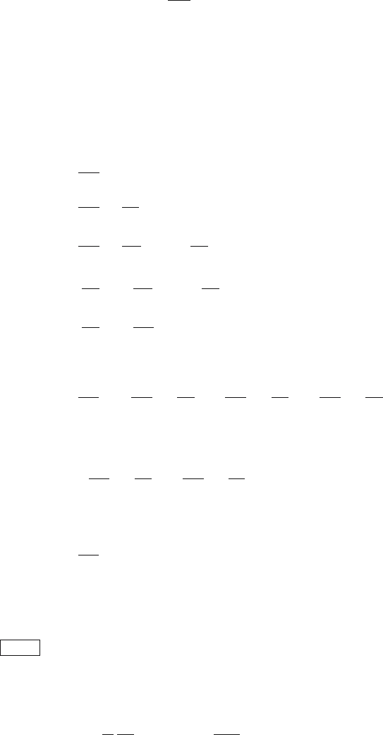
Fig. 8.1 shows optimal trajectories of u(t)andx(t)fort
f
= ∞, x
0
=1,
r =1.
8.2 Feedback Optimal Control
Optimal control of processes presented in Section 8.1 can also be implemented
using the feedback configuration.
The problem of optimal feedback control of a linear time-invariant dynamic
system can be formulated as follows.
Consider a completely controllable system
˙x(t)=Ax(t)+Bu(t) (8.39)
with initial condition at time t
0
=0
x(0) = x
0
(8.40)
and terminal condition x(t
f
), t
f
. We assume that t
f
is fixed.
306 8 Optimal Process Control
0 1 2 3 4
−0.5
0
0.5
1
t
u
*
, x
*
u
*
x
*
Fig. 8.1. Optimal trajectories of input and state variables of the heat exchanger
The cost function is defined as
I =
1
2
x
T
(t
f
)Q
t
f
x(t
f
)+
1
2
t
f
0
x
T
(t)Qx(t)+u
T
(t)Ru(t)
dt (8.41)
where Q
t
f
and Q are real symmetric positive semidefinite weighting matrices
and R is a real symmetric positive definite weighting matrix.
Our aim is to find a feedback control law of the form
u = function(x) (8.42)
such that I be minimal for any initial condition x
0
.
Optimal feedback control guarantees the change of the operating point
within t ∈ [0,t
f
] from state x
0
to a neighbourhood of the origin x = 0.
Hamiltonian is for our case defined as
H =
1
2
(x
T
Qx + u
T
Ru)+λ
T
(Ax + Bu) (8.43)
where the adjoint vector λ(t) satisfies the differential equation
˙
λ = −Qx −A
T
λ (8.44)
with terminal condition

8.2 Feedback Optimal Control 307
λ(t
f
)=Q
t
f
x(t
f
) (8.45)
If there are no constraints on u(t) then the optimal control condition can
be written as
Ru + B
T
λ = 0 (8.46)
Optimal control u is then given as
u(t)=−R
−1
B
T
λ(t) (8.47)
The matrix R
−1
exists as R is square symmetric positive definite matrix.
Optimal control has to minimise the Hamiltonian. The necessary condition
∂H/∂u only specifies an extremum. To assure minimum for u, the second
partial derivative with respect to control ∂
2
H/∂u
2
with dimensions m × m
needs to be positive definite. From (8.46) follows
∂
2
H
∂u
2
= R (8.48)
As R is assumed to be positive definite, the optimal control (8.47) indeed
minimises the Hamiltonian.
Substitute now u(t) from (8.47) to (8.39)
˙x(t)=Ax(t) −BR
−1
B
T
λ(t) (8.49)
Let us denote
S = BR
−1
B
T
(8.50)
Matrix S has dimensions n × n. Equations (8.49), (8.44) can now be written
as
⎛
⎝
˙x(t)
−−
˙
λ(t)
⎞
⎠
=
⎛
⎝
A |−S
−− −− −−
−Q |−A
T
⎞
⎠
⎛
⎝
x(t)
−−
λ(t)
⎞
⎠
(8.51)
This represents 2n of linear differential equations with constant coefficients.
Its solution can be found if 2n initial conditions are known. In our case there
are n initial conditions x(0) = x
0
and n terminal conditions on the adjoint
vector given by (8.45).
Let Φ(t, t
0
) be the state transition matrix of the system (8.51) with di-
mensions 2n ×2n and t
0
=0.Ifλ(0) denotes the unknown initial value of the
adjoint vector, the solution of (8.51) is of the form
x(t)
λ(t)
= Φ(t, t
0
)
x(t
0
)
λ(t
0
)
(8.52)
At t = t
f
it holds
308 8 Optimal Process Control
x(t
f
)
λ(t
f
)
= Φ(t
f
,t)
x(t)
λ(t)
(8.53)
Let us divide the matrix Φ(t
f
,t) to four matrices of dimensions n ×n
Φ(t
f
,t)=
⎛
⎝
Φ
11
(t
f
,t) | Φ
12
(t
f
,t)
−−−−−|−−−−
Φ
21
(t
f
,t) | Φ
22
(t
f
,t)
⎞
⎠
(8.54)
Equation (8.53) can now be written as
x(t
f
)=Φ
11
(t
f
,t)x(t)+Φ
12
(t
f
,t)λ(t) (8.55)
λ(t
f
)=Φ
21
(t
f
,t)x(t)+Φ
22
(t
f
,t)λ(t)=Q
t
f
x(t
f
) (8.56)
After some manipulations from (8.55) and (8.56) follows
λ(t)=[Φ
22
(t
f
,t) −Q
t
f
Φ
12
(t
f
,t)]
−1
[Q
t
f
Φ
11
(t
f
,t) −Φ
21
(t
f
,t)]x(t) (8.57)
provided that the inverse matrix in (8.57) exists. Equation (8.57) says that
the adjoint vector λ(t) and the state vector x(t) are related as
λ(t)=P (t)x(t) (8.58)
where
P (t)=[Φ
22
(t
f
,t) −Q
t
f
Φ
12
(t
f
,t)]
−1
[Q
t
f
Φ
11
(t
f
,t) −Φ
21
(t
f
,t)] (8.59)
Equation (8.58) determines the function (8.42) of the optimal feedback
control law minimising the cost function I
u(t)=−R
−1
B
T
P (t)x(t) (8.60)
It can be proved that P (t) exists for any time t where t
0
≤ t ≤ t
f
. However,
to determine P (t) from (8.59) is rather difficult. Another possibility of finding
it is to derive a differential equation with solution P (t). This equation will be
derived as follows.
Suppose that solutions of (8.51) are tied together by equation (8.58) for
t ∈t
0
,t
f
.
Differentiating (8.58) with respect to time yields
˙
λ(t)=
˙
P (t)x(t)+P (t) ˙x(t) (8.61)
Substituting u(t) from (8.47) and λ(t) from (8.58) into (8.39) gives
˙x(t)=Ax(t) −BR
−1
B
T
P (t)x(t) (8.62)
Equations (8.61), (8.62) give
˙
λ(t)=[
˙
P (t)+P (t)A − P (t)BR
−1
B
T
P (t)]x(t) (8.63)

8.2 Feedback Optimal Control 309
From (8.44) and (8.58) yields
˙
λ(t)=[−Q −A
T
P (t)]x(t) (8.64)
Equating the right-hand sides of (8.63) and (8.64) gives the relation
[
˙
P (t)+P (t)A −P (t)BR
−1
B
T
P (t)+A
T
P (t)+Q]x(t)=0,t∈t
0
,t
f
(8.65)
As the vector x(t) is a solution of the homogeneous equation (8.62), matrix
P (t) obeys the following differential equation
dP (t)
dt
+ P (t)A + A
T
P (t) −P (t)BR
−1
B
T
P (t)=−Q (8.66)
Comparing the expression
λ(t
f
)=P (t
f
)x(t
f
) (8.67)
and expression (8.45) yields a terminal condition needed to solve equa-
tion (8.66) of the form
P (t
f
)=Q
t
f
(8.68)
Equation (8.66) is a Riccati matrix differential equation. Its solution exists
and is unique. It can be shown that the matrix P (t) is positive definite and
symmetric
P (t)=P
T
(t) (8.69)
Further, optimal control for the system (8.39) exists and is unique for the cost
function (8.41). It is given by the equation
u(t)=−K(t)x(t) (8.70)
where
K(t)=R
−1
B
T
P (t) (8.71)
It is important to realise that the matrix P (t) can be calculated before-
hand.
Controllability of the system (8.39) is not the necessary condition for the
fact that the optimal control is given by the control law (8.70). This is because
the influence of uncontrollable elements in the cost function I is always finite
if the time interval of optimisation is finite. If, on the other hand, the final
time t
f
goes to infinity, controllability is required to guarantee the finite value
of I.
Example 8.2: Optimal feedback control of a heat exchanger
www
310 8 Optimal Process Control
Consider the heat exchanger from Example 8.1 and the problem of its
optimal feedback control. The system state-space matrices are A = −1,
B = 1 and the cost function is defined by Q
t
f
=0,Q =2,R =2r
= r.
Optimal feedback control is given as
u(t)=−
1
r
P (t)x(t)
where P (t) is the solution of the differential equation of the form
dP (t)
dt
− 2P(t) −
P
2
(t)
r
= −2
with terminal condition
P (t
f
)=0
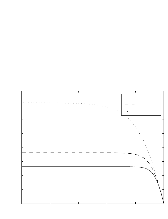
Fig. 8.2 shows trajectories of P for various values of r if t
f
=1.
0 0.2 0.4 0.6 0.8 1
0
0.05
0.1
0.15
0.2
0.25
0.3
0.35
0.4
t
P
r = 0.01
r = 0.02
r = 0.10
Fig. 8.2. Trajectories of P (t) for various values of r
Example 8.2 shows a very important fact. If the matrix Riccati equation
starts at time t
f
= ∞ then its solutions given by elements of matrix P (t)
will be constant. Such a matrix P containing steady-state solution of the
differential matrix Riccati equation can be used in optimal control for all
finite times with initial time equal to t =0.