Mikles J., Fikar M. Process Modelling, Identification, and Control
Подождите немного. Документ загружается.

8.2 Feedback Optimal Control 311
Therefore, optimal control design can be simplified considerably in the case
of infinite final time as it is shown below.
Consider the system (8.39) with the initial condition (8.40) and the cost
function
I =
1
2
∞
0
x
T
(t)Qx(t)+u
T
(t)Ru(t)
dt (8.72)
where Q is a real symmetric positive semidefinite weighting matrix and R is
a real symmetric positive definite weighting matrix.
Solution of the optimisation problem, i. e. minimisation of I for any x
0
satisfies the feedback control law
u(t)=−Kx(t) (8.73)
where
K = R
−1
B
T
P (8.74)
and where P is a symmetric positive semidefinite solution of the matrix Riccati
equation
PA+ A
T
P − PBR
−1
B
T
P = −Q (8.75)
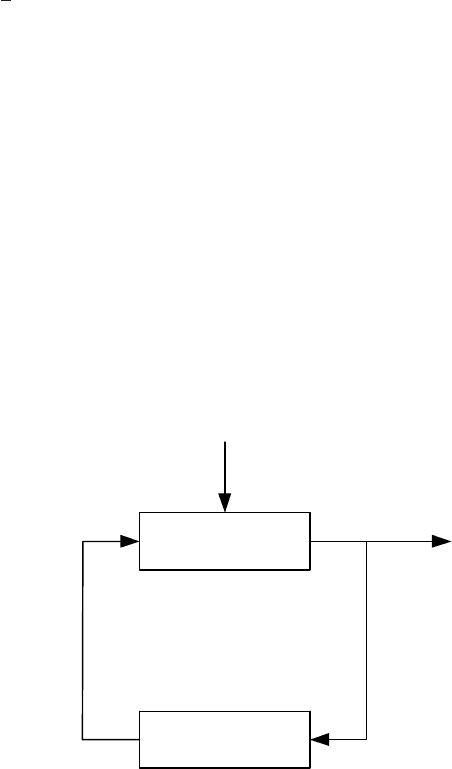
x = Ax + Bu
-K
.
x
0
x
u
Fig. 8.3. Optimal feedback control
Equation (8.73) is easily implementable. It is a feedback control law. As
K is a constant matrix, the controller implements proportional action. This
controller is called Linear Quadratic Regulator (LQR). This says that the
controlled system is linear, the cost function is quadratic and the controller
312 8 Optimal Process Control
regulates the system in the neighbourhood of the setpoint x
w
= 0.Block
scheme of feedback LQR control is shown in Fig. 8.3.
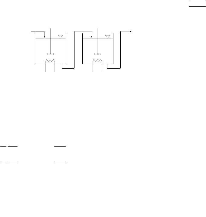
Example 8.3: Optimal feedback control of two heat exchangers in series
www
Consider two heat exchangers (Fig. 8.4) where a liquid is heated.
1
ϑ
0
ϑ
ω
1
ω
2
1
ϑ
2
ϑ
V
2
V
1
2
ϑ
q
q
Fig. 8.4. Two heat exchangers in series
Assume that heat flows from heat sources into liquid are independent
from liquid temperature. Further assume an ideal liquid mixing and zero
heat losses. We neglect accumulation ability of exchangers walls. Hold-
ups of exchangers, as well as flow rates and liquid specific heat capacity
are constant. Under these assumptions the mathematical model of the
exchangers is given as
V
1
q
dϑ
1
dt
+ ϑ
1
= ϑ
0
+
ω
1
qρc
p
V
2
q
dϑ
2
dt
+ ϑ
2
= ϑ
1
+
ω
2
qρc
p
where ϑ
1
is temperature in the first exchanger, ϑ
2
– temperature in the
second exchanger, t
– time, ϑ
0
– liquid temperature in the first tank inlet
stream, ω
1
,ω
2
– heat input, q – volumetric flowrate of liquid, ρ – liquid
density, V
1
,V
2
– liquid volume, c
p
– specific heat capacity.
Denote
ϑ
u1
=
ω
1
qρc
p
,ϑ
u2
=
ω
2
qρc
p
,T
1
=
V
1
q
,T
2
=
V
2
q
ϑ
u1
,ϑ
u2
are in temperature units and T
1
, T
2
are time constants. The
process inputs are temperatures ϑ
0
,ϑ
u1
,andϑ
u2
. The state variables are
ϑ
1
and ϑ
2
. Temperature ϑ
u1
will be assumed as the manipulated variable.
Assume that the manipulated input is constant for a sufficiently long
time and equal to ϑ
u10
. If the inlet temperature to the first exchanger
is constant ϑ
0
= ϑ
00
and the heat input to the second exchanger will
be constant as well (ϑ
u2
= ϑ
u20
) then the heat exchangers will be in a
steady-state described by equations
ϑ
10
= ϑ
00
+ ϑ
u10
,ϑ
20
= ϑ
10
+ ϑ
u20
8.2 Feedback Optimal Control 313
Let us now assume a new steady-state characterised by the manipulated
variable ϑ
u11
defined by equations
ϑ
11
= ϑ
00
+ ϑ
u11
,ϑ
21
= ϑ
11
+ ϑ
u20
The problem of optimal control is now to find a way to shift the system in
the original steady-state with the manipulated variable ϑ
u10
to the new
steady-state with ϑ
u11
in such a way that some cost function be minimal.
At first we define new state variables as dimensionless deviation variables
from the final steady-state
x
1
(t
)=
ϑ
1
(t
) −ϑ
11
ϑ
u11
− ϑ
00
x
2
(t
)=
ϑ
2
(t
) −ϑ
21
ϑ
u20
− ϑ
11
A new manipulated variable is defined as
u
1
(t
)=
ϑ
u1
(t
) −ϑ
u11
ϑ
u11
− ϑ
00
Further, a dimensionless time variable is given as
t =
q
V
1
t
This gives for the heat exchanger model
dx
1
(t)
dt
+ x
1
(t)=u
1
(t)
k
1
dx
2
(t)
dt
+ x
2
(t)=k
2
x
1
(t)
where k
1
= V
2
/V
1
a k
2
=(ϑ
u11
− ϑ
00
)/(ϑ
u20
− ϑ
11
).
Transformed initial conditions are given as
x
1
(0) = x
10
=
ϑ
10
− ϑ
11
ϑ
u11
− ϑ
00
x
2
(0) = x
20
=
ϑ
20
− ϑ
21
ϑ
u20
− ϑ
11
Let us now design an optimal feedback controller that minimises the cost
function
I =
1
2
∞
0
x
T
(t) Qx(t)+ru
1
(t)
dt
where x =(x
1
x
2
)
T
Q =
q
11
0
0 q
22
, R = r
The controlled system is defined as

314 8 Optimal Process Control
A =
⎛
⎝
−10
k
2
k
1
−
1
k
1
⎞
⎠
, B =
1
0
Optimal feedback is thus given as
u
1
(t)=−
1
r
B
T
Px(t)
and P is solution of the equation
PA+ A
T
P − PBR
−1
B
T
P = −Q
where
P =
p
11
p
12
p
12
p
22
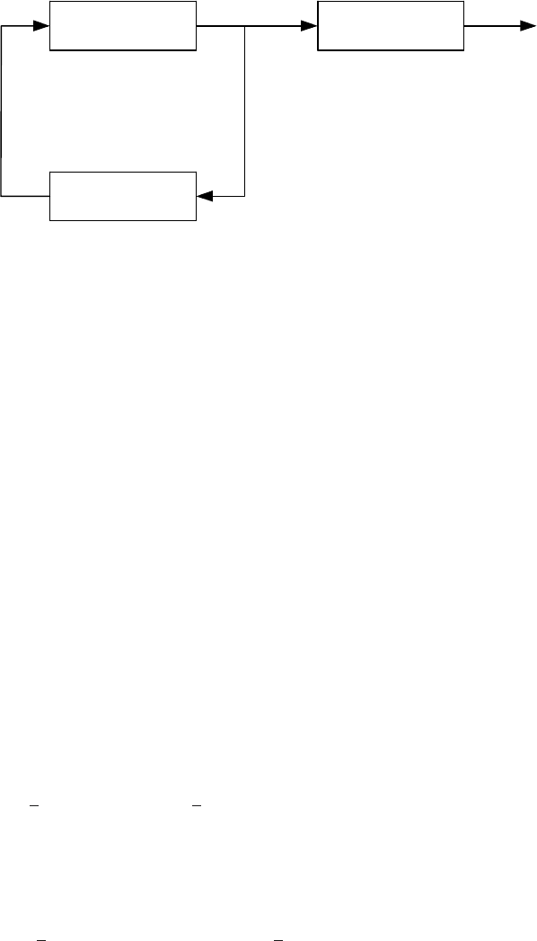
Fig. 8.6 shows optimal trajectories x
1
, x
2
,andu
1
of the heat exchangers
(Fig. 8.4) for k
1
=1,k
2
= −1/5, q
11
= q
22
=1,andr =1.
Matrix
K =(k
11
k
12
)=
1
r
(p
11
p
12
)
was calculated using MATLAB (program 8.1) and trajectories x
1
, x
2
,and
u
1
in Fig. 8.6 were obtained from SIMULINK program shown in Fig. 8.5
with initial conditions x
10
=1,x
20
= −1/3.
Program 8.1 (Program to calculate LQ gains for Example 8.3)
% LQR feedback for the heat exchanger
% program: lqvym2rm.m
x0 = [1;-1/3];
A = [-1 0; -0.2 -1];
B = [1; 0];
C=eye(2);
D=zeros(2,1);
Q=eye(2);
R=1;
[K,S,E]=LQR(A,B,Q,R);
Consider now the system shown in Fig. 8.3. It is described by
˙x(t)=Ax(t) −BKx(t) (8.76)

8.2 Feedback Optimal Control 315
x
x
u
u
lqvym2rm
lqvym2rm
x’ = Ax+Bu
y = Cx+Du
System
Scope x
Scope u
K
Matrix
Gain
−1
Gain
Fig. 8.5. Simulink program to simulate feedback optimal control in Example 8.3
0 1 2 3 4 5 6
−0.5
0
0.5
1
t
u, x
u
x
1
x
2
Fig. 8.6. LQ optimal trajectories x
1
, x
2
, u
1
of heat exchangers

316 8 Optimal Process Control
with initial condition at time t
0
=0
x(0) = x
0
(8.77)
where K = R
−1
B
T
P and P is the solution of (8.75).
Equation (8.76) can also be written as
˙x(t)=(A −BK) x(t), x(0) = x
0
(8.78)
The transition matrix of the closed-loop system is given as
¯
A = A −BK (8.79)
The system (8.78) is solution of the optimisation problem based on min-
imisation of the cost function (8.72). This cost function can be written as
I =
1
2
∞
0
x
T
(t)Qx(t)+x
T
(t)K
T
RKx(t)
dt (8.80)
or
I =
1
2
∞
0
x
T
(t)
Q + K
T
RK
x(t)dt (8.81)
and can also be formulated as follows
I =
1
2
∞
0
x
T
0
e
¯
A
T
t
¯
Qe
¯
At
x
0
dt (8.82)
or
I =
1
2
x
T
0
Px
0
(8.83)
where
¯
Q = Q + K
T
RK (8.84)
and
P =
∞
0
e
¯
A
T
t
¯
Qe
¯
At
dt (8.85)
Matrix P can be integrated by parts yielding
P =e
¯
A
T
t
¯
Q
¯
A
−1
e
¯
At
∞
0
−
∞
0
¯
A
T
e
¯
A
T
t
¯
Q
¯
A
−1
e
¯
A
T
t
dt (8.86)
If matrix
¯
A is stable then
P = −
¯
Q
¯
A
−1
−
¯
A
T
∞
0
e
¯
A
T
t
¯
Qe
¯
At
dt
¯
A
−1
(8.87)

8.3 Optimal Tracking, Servo Problem, and Disturbance Rejection 317
and after some manipulations
¯
A
T
P + P
¯
A = −
¯
Q (8.88)
This is the Lyapunov equation. It is known that for an arbitrary symmetric
positive definite matrix
¯
Q there a is symmetric positive definite matrix P that
is solution of this equation if matrix
¯
A is asymptotically stable.
When
¯
A is back-substituted into (8.88) from (8.79) and
¯
Q from (8.84),
then we obtain
(A −BK)
T
P + P (A − BK)=−Q −
R
−1
B
T
P
T
R
R
−1
B
T
P
(8.89)
This equation can be easily rewritten to the form (8.75).
It is important to observe that the optimal feedback control shown in
Fig. 8.3 places optimally poles of the closed-loop system.
Pole Placement (PP) represents such feedback control design where the
matrix K in (8.79) is chosen so that the matrix
¯
A is asymptotically stable.
LQR control is in this aspect only a special case of the PP control design.
Consider now a system
˙x(t)=Ax(t)+Bu(t), x(0) = x
0
(8.90)
y(t)=Cx(t) (8.91)
and cost function
I =
1
2
∞
0
y
T
(t)Q
y
y(t)+u
T
(t)Ru(t)
dt (8.92)
Substituting equation (8.91) into (8.92) yields
I =
1
2
∞
0
x
T
(t)C
T
Q
y
Cx(t)+u
T
(t)Ru(t)
dt (8.93)
Denote as
Q = C
T
Q
y
C (8.94)
then the cost function (8.93) is of the same form as (8.72) and the output
regulation problem has been transformed into the classical LQR problem. So-
lution of the optimal problem, i. e. minimisation of I from (8.93) for arbitrary
x
0
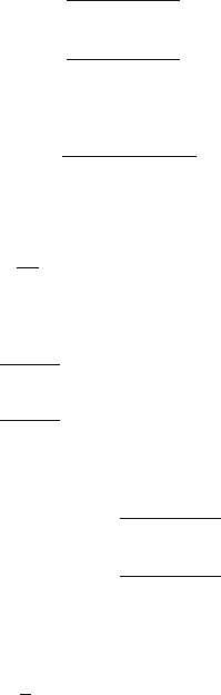
guarantees the state feedback given by equation (8.73). The block diagram
of output LQR is shown in Fig. 8.7.
8.3 Optimal Tracking, Servo Problem, and Disturbance
Rejection
Previous section was devoted to the problem when a system was to be steered
from some initial state to a new state in some optimal way. In fact, this is
only a special case of a general problem of optimal setpoint tracking.
318 8 Optimal Process Control
x = Ax + Bu
-K
.
y = Cx
xyu
Fig. 8.7. Optimal LQ output regulation
The tracking problem of some desired trajectories can be divided into two
subproblems. If desired trajectories are prescribed functions of time then we
speak about the tracking problem. If the process outputs should follow some
class of desired trajectories then we speak about the servo problem.
LQ design leads to a proportional feedback control. However, such design
results in the steady-state control error if setpoint changes or disturbances
occur. If the zero steady-state control error is desired, it is necessary to modify
the controller with integral action.
8.3.1 Tracking Problem
Consider a controllable and observable linear system
˙x(t)=Ax(t)+Bu(t), x(0) = x
0
(8.95)
y(t)=Cx(t) (8.96)
Let w(t) be a vector of setpoint variables of dimensions r. Our aim is to
control the system in such a way that the control error vector
e(t)=w(t) −y(t) (8.97)
should be “close” to zero with a minimum control effort.
The cost function that is to be minimised is of the form
I =
1
2
e
T
(t
f
)Q
yt
f
e(t
f
)+
1
2
t
f
0
e
T
(t)Q
y
e(t)+u
T
(t)Ru(t)
dt (8.98)
Assume that t
f
is fixed, Q
yt
f
and Q
y
are real symmetric positive semidefinite
matrices, R is a real symmetric positive definite matrix.
Hamiltonian is of the form
H =
1
2
(w − Cx)
T
Q
y
(w − Cx)+
1
2
u
T
Ru + λ
T
(Ax + Bu) (8.99)
8.3 Optimal Tracking, Servo Problem, and Disturbance Rejection 319
Optimality condition
∂H
∂u
= 0
gives
u(t)=−R
−1
B
T
λ(t) (8.100)
Adjoint vector λ(t) is the solution of the differential equation
˙
λ = −
∂H
∂x
or
dλ(t)
dt
= C
T
Q
y
(w(t) −Cx(t)) −A
T
λ(t) (8.101)
Similarly, as (8.58) was derived, we can write
λ(t)=P (t)x(t) −γ(t) (8.102)
Derivative of (8.102) with respect to time gives
dλ(t)
dt
=
dP (t)
dt
x(t)+P (t)
dx(t)
dt
−
dγ(t)
dt
(8.103)
From (8.95) and (8.100) follows
˙x(t)=Ax(t) −BR
−1
B
T
λ(t) (8.104)
Substituting for λ(t) from (8.102) gives
˙x(t)=Ax(t) −BR
−1
B
T
P (t)x(t)+BR
−1
B
T
γ(t) (8.105)
Differential equation (8.103) can now be written as
˙
λ(t)=
˙
P (t)+P (t)A − P (t)BR
−1
B
T
P (t)
x(t)+PBR
−1
B
T
γ(t)−
˙
γ(t)
(8.106)
This can be simplified using (8.101) and (8.102) as
˙
λ(t)=
−C
T
Q
y
C − A
T
P (t)
x(t)+A
T
γ(t)+C
T
Q
y
w(t) (8.107)
As the optimal solution exists, equations (8.106) and (8.107) hold for any x(t)
and w(t). From this follows that matrix P (t) with dimensions n × n has to
satisfy the equation
˙
P (t)=−P (t)A − A
T
P (t)+P (t)BR
−1
B
T
P (t) − C
T
Q
y
C (8.108)

320 8 Optimal Process Control
Further, for vector γ(t) with dimension n holds
˙γ(t)=
P (t)BR
−1
B
T
− A
T
γ(t) −C
T
Q
y
w(t) (8.109)
Final conditions for the adjoint variables are specified by (8.102)
λ(t
f
)=P (t
f
)x(t
f
) −γ(t
f
) (8.110)
and the principle of minimum gives
λ(t
f
)=
∂
∂x(t
f
)
1
2
e
T
(t
f
)Q
yt
f
e(t
f
)
(8.111)
= C
T
Q
yt
f
Cx(t
f
) −C
T
Q
yt
f
w(t
f
) (8.112)
Equations (8.110) and (8.112) hold for any x(t
f
)andw(t
f
). Thus
P (t
f
)=C
T
Q
yt
f
C (8.113)
γ(t
f
)=C
T
Q
yt
f
w(t
f
) (8.114)
The optimal state trajectory is defined by solution of linear differential equa-
tion (8.105).
The control law can be written as
u(t)=R
−1
B
T
[γ(t) −P (t)x(t)] (8.115)
Symmetric positive definite matrix P (t) with dimension n × n is solution
of (8.108) with terminal condition (8.113). Vector γ(t) with dimension n is
solution of (8.109) with terminal condition (8.114).
To calculate γ(t), vector w(t) is needed in the entire interval [0,t
f
]. This
is a rather impractical condition. However, if w(t)=0andt
f
→∞optimal
control law is described by (8.73) where matrix P is given by (8.75) where
Q = C
T
QC.
8.3.2 Servo Problem
Consider now an optimal feedback control where the desired vector of output
variables is generated as
˙x
w
(t)=A
w
x
w
(t), x
w
(0) = x
w0
(8.116)
w(t)=C
w
x
w
(t) (8.117)
We want to ensure that y(t) is “close” to w(t) with minimal control effort.
This problem can mathematically be formulated as minimisation of the cost
function
I =
∞
0
(y(t) −w(t))
T
Q
y
(y(t) −w(t)) + u
T
(t)Ru(t)
dt (8.118)
Substituting y(t) from (8.96) and w(t) from (8.117) into the cost gives