Mikles J., Fikar M. Process Modelling, Identification, and Control
Подождите немного. Документ загружается.

8.3 Optimal Tracking, Servo Problem, and Disturbance Rejection 321
I =
∞
0
(Cx(t) −C
w
x
w
(t))
T
Q
y
(Cx(t) −C
w
x
w
(t)) + u
T
(t)Ru(t)
dt
(8.119)
or, after some manipulations
I =
∞
0
x
T
(t) x
T
w
(t)
C
T
Q
y
C −C
T
Q
y
C
w
−C
T
w
Q
y
CC
T
w
Q
y
C
w
x(t)
x
w
(t)
+ u
T
(t)Ru(t)
dt (8.120)
To solve the optimal control problem, an expanded controlled system is
assumed
˙x(t)
˙x
w
(t)
=
A 0
0 A
w
x(t)
x
w
(t)
+
B
0
u(t) (8.121)
From previous derivations follows that the solution of this problem leads
to the Riccati equation of the form
A 0
0 A
w
P + P
A 0
0 A
w
− P
B
0
R
−1
B
0
T
P
= −
C
T
Q
y
C −C
T
Q
y
C
w
−C
T
w
Q
y
CC
w
Q
y
C
w
(8.122)
If matrix P is decomposed into
P =
P
11
P
12
P
21
P
22
(8.123)
then the optimal control law is given as
u(t)=−R
−1
B
T
[P
11
x(t)+P
12
x
w
(t)]
8.3.3 LQ Control with Integral Action
LQ control results in proportional feedback controller. This leads to the
steady-state control error in case of setpoint changes or disturbances. There
are two possible ways to add integral action to the closed-loop system and to
remove the steady-state error.
In the first case the LQ cost function is modified and vector u(t) is replaced
by its time derivative ˙u(t).
Another possibility is to add new states acting as integrators to the closed-
loop system. The number of integrators is equal to the dimension of the control
error.

322 8 Optimal Process Control
8.4 Dynamic Programming
8.4.1 Continuous-Time Systems
Bellman with his coworkers developed around 1950 a new approach to system
optimisation – dynamic programming. This method is often used in analysis
and design of automatic control systems.
Consider the vector differential equation
dx(t)
dt
= f(x(t), u(t),t) (8.124)
where f and x are of dimension n, vector u is of dimension m. The control
vector u is within a region
u ∈ U (8.125)
where U is a closed part of the Euclidean space E
m
.
The cost function is given as
I =
t
f
t
0
F (x(t), u(t),t)dt (8.126)
The terminal time t
f
>t
0
can be free of fixed. We will consider the case with
fixed time.
Let us define a new state variable
x
n+1
(t)=
t
t
0
F (x(τ), u(τ ),τ)dτ (8.127)
The problem of minimisation of I is equivalent to minimisation of the state
x
n+1
(t
f
) of the system described by equations
d˜x(t)
dt
=
˜
f (˜x(t), u(t),t) (8.128)
where
˜x
T
=
x
T
,x
n+1
˜
f
T
=
f
T
,F
and with initial conditions
˜x
T
(t
0
)=
x
T
(t
0
), 0
(8.129)
This includes the time optimal control with F =1.
If a direct presence of time t in (8.124) is undesired, it is possible to intro-
duce a new state variable x
0
(t)=t and a new differential equation
8.4 Dynamic Programming 323
dx
0
(t)
dt
= 1 (8.130)
with initial condition x
0
(t
0
) = 0. The new system of differential equations is
then defined as
dx(t)
dt
= f (x(t), u(t)) (8.131)
1
x
2
x
n
x
)(
0
tx
)(
f
tx
)'(tx
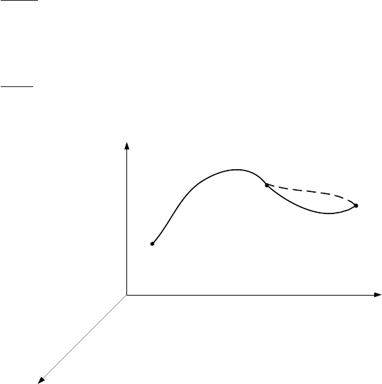
Fig. 8.8. Optimal trajectory in n-dimensional state space
Dynamic programming is based on the principle of optimality first for-
mulated by Bellman. Let us consider the optimal trajectory in n-dimensional
state space (Fig. 8.8). Position of moving point in time t = t
(t
0
<t
<t
f
)
will be denoted by x(t
). This point divides the trajectory into two parts.
The principle of optimality states that any part of the optimal trajectory
from point x(t
) to point x(t
f
) is optimal. From this follows that for the initial
point x(t
) the second part of the trajectory between points x(t
)andx(t
f
)
is optimal and does not depend on the system history, i. e. the way how the
point x(t
) was reached. Suppose now that this does not hold, i. e. we find a
trajectory (shown in Fig. 8.8 by dashed line), where the cost function value
is smaller. The overall cost function value is given as the sum of values in the
both trajectory parts. This means that it is possible to find a better trajectory
than the original. To do so, it is necessary to find a control vector trajectory
in such a way that the first part of the state trajectory remains the same and
the second coincides with the dashed line. This is in contradiction with the
assumption that the original trajectory is optimal. Therefore, it is not possible
to improve the second part of the trajectory and it is optimal as well.
324 8 Optimal Process Control
The principle of optimality makes it possible to obtain general conditions
of optimisation that are valid for both continuous-time and discrete-time sys-
tems. Although its formulation is very simple, we can derive the necessary
optimisation conditions.
The principle of optimality can alternatively be formulated as follows:
optimal trajectory does not depend on previous trajectory and is determined
only by the initial condition and the terminal state.
Based on the principle of optimality, determination of the optimal trajec-
tory is started at the terminal state x(t
f
). We stress again that the trajectory
that ends in the optimal terminal state is optimal. In other words, optimality
of one part depends on the optimality of the entire trajectory.
We can check optimality of the last part of the trajectory and after that
the optimality of preceding parts. Optimality of partial trajectories depends
on the optimality of the entire trajectory. The opposite statement does not
hold, i. e. the optimality of the overall trajectory does not follow from the
optimality of partial trajectories.
1
x
2
x
n
x
)(
0
tx
)(
f
tx
)(
*
tx
)()'(
**
ttt Δ+= xx
Fig. 8.9. Optimal trajectory
Consider a vector differential equation of a non-linear controlled object of
the form
dx(t)
dt
= f (x(t), u(t),t) (8.132)
The cost function to be minimised is given as
I =
t
f
t
0
F (x(t), u(t),t)dt (8.133)

8.4 Dynamic Programming 325
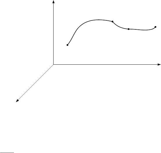
Suppose that x
∗
(t) is the optimal trajectory with the initial state x(t
0
)and
terminal state x(t
f
) (Fig. 8.9). Denote by I
∗
(x
∗
(t
0
),t
0
) minimum of the cost
function I. It follows from the principle of optimality that the part of the
trajectory with the initial state x
∗
(t), terminal state x(t
f
) and that satisfies
equation (8.132) is optimal as well.
From this follows that
I
∗
(x
∗
(t),t) = min
u∈U
t
f
t
F (x
∗
(τ), u(τ ),τ)dτ (8.134)
This is Bellman’s functional equation. For a sufficiently small interval Δt and
time t
= t +Δt, the minimum value of the cost function on the interval
x
∗
(t
)=x
∗
(t +Δt), x(t
f
) is given as
I
∗
(x
∗
(t
),t
) = min
u∈U
t
f
t
F (x
∗
(τ), u(τ ),τ)dτ (8.135)
The arguments x
∗
(t
), t
of the left hand side of equation (8.135) denote initial
state of the given trajectory. Comparing integrals (8.134) and (8.135) gives
I
∗
(x
∗
(t),t) = min
u∈U
t
f
t
F (x
∗
(τ), u(τ ),τ)dτ + F (x
∗
(t), u(t),t)Δt
+ o
1
(Δt) (8.136)
= min
u∈U
{I
∗
(x
∗
(t
),t
)+F (x
∗
(t), u(t),t)Δt} + o
1
(Δt)
(8.137)
where o
1
(Δt) is a remainder satisfying
lim
Δt→0
o
1
(Δt)
Δt
= 0 (8.138)
The remainder is nonzero because the interval Δt has a finite value in the
right hand parts of equations (8.136), (8.137).
The Taylor expansion gives
x(t
)=x (t +Δt)=x(t)+ ˙x(t)Δt + o
2
(Δt) (8.139)
where o
2
(Δt) is a remainder. Taking (8.132) into account gives
x(t
)=x(t)+f (x(t), u(t),t)Δt + o
2
(Δt) (8.140)
Substituting x(t
) from (8.140) into I
∗
(x(t
),t
) and applying the Taylor ex-
pansion (assuming that partial derivatives ∂I
∗
/∂x
i
,(i =1, 2,...,n), ∂I
∗
/∂t
exist) gives

326 8 Optimal Process Control
I
∗
(x(t
),t
)=I
∗
(x (t +Δt) ,t+Δt) (8.141)
= I
∗
{x(t)+f (x(t), u(t),t)Δt + o
2
(Δt) ,t+Δt} (8.142)
= I
∗
(x(t),t)+
n
i=1
∂I
∗
(x(t),t)
∂x
i
f
i
(x(t), u(t),t)Δt
+
∂I
∗
(x(t),t)
∂t
Δt + o
3
(Δt) (8.143)
where o
3
(Δt) is a remainder. Denote as
∂I
∗
∂x
=
∂I
∗
∂x
1
,
∂I
∗
∂x
2
, ··· ,
∂I
∗
∂x
n
T
(8.144)
then equation (8.143) can be rewritten as
I
∗
(x(t
),t
)=I
∗
(x(t),t)
+
∂I
∗
(x(t),t)
∂x
T
f (x(t), u(t),t)Δt +
∂I
∗
(x(t),t)
∂t
Δt + o
3
(Δt) (8.145)
This expression is substituted into the right hand side of equation (8.137) as-
suming that x(t)=x
∗
(t). As expressions I
∗
(x(t),t), ∂I
∗
/∂t do not depend on
u(t) they can be taken out before the operator min. Simplifying the expression
and dividing the equation by Δt yields
−
∂I
∗
(x
∗
(t),t)
∂t
=
min
u∈U
∂I
∗
(x
∗
(t),t)
∂x
∗T
f (x
∗
(t), u(t),t)+F (x
∗
(t), u(t),t)
+
o
4
(Δt)
Δt
(8.146)
where o
4
(Δt) is a remainder. If Δt → 0, the last term on the right hand of
the equation vanishes. This gives the Hamilton-Jacobi equation (or Hamilton-
Jacobi-Bellman (HJB) equation)
−
∂I
∗
(x
∗
(t),t)
∂t
=
min
u∈U
∂I
∗
(x
∗
(t),t)
∂x
∗T
f (x
∗
(t), u(t),t)+F (x
∗
(t), u(t),t)
(8.147)
This is the basic equation of dynamic programming for continuous-time
systems. The first part is independent on control u(t) after minimisation. The
equation holds only for optimal control u
∗
(t). HJB equation is often used in
the form
−
∂I
∗
(x
∗
(t),t)
∂t
=
∂I
∗
(x
∗
(t),t)
∂x
∗T
f (x
∗
(t), u
∗
(t),t)+F (x
∗
(t), u
∗
(t),t)
(8.148)

8.4 Dynamic Programming 327
As (∂I
∗
/∂t+(∂I
∗
/∂x
T
)f) is equal to dI
∗
/dt, the equation can also be written
as
dI
∗
(x
∗
(t),t)
dt
+ F (x
∗
(t), u
∗
(t),t) = 0 (8.149)
Similarly, the basic HJB equation (8.147) can be written as
min
u∈U
dI
∗
(x
∗
(t),t)
dt
+ F (x
∗
(t), u
∗
(t),t)
= 0 (8.150)
The Hamilton-Jacobi-Bellman equation (8.147) or (8.150) specifies necessary
optimality conditions. Under some assumptions can sufficent conditions be
formulated similarly.
We will now show that optimal control described by the equation (8.70) is
unique.
The proof is based on the fact that the solution of the Riccati equation
P (t) with terminal condition P (t)=Q
t
f
is unique.
If the optimal control exists then it is unique and determined by equa-
tion (8.70).
If the matrix P (t) is unique then the optimal control is the unambiguos
function of the state. Suppose that there are two optimal control trajectories
u
1
(t), u
2
(t) and two optimal state trajectories x
1
(t), x
2
(t) with x
1
(t
0
)=
x
2
(t
0
). Vectors x
1
(t), x
2
(t) are two different solutions of the equation
dx(t)
dt
=
A −BR
−1
B
T
P (t)
x(t) (8.151)
and x
1
(t
0
)=x
2
(t
0
). As the matrix P (t) is unique, the same holds for matrix
(A − BR
−1
B
T
P ). Equation (8.151) is linear and homogenous, therefore its
solution is unique. It follows that x
1
(t)=x
2
(t), u
1
(t)=u
2
(t) in any time
t ∈t
0
,t
f
.
The next theorem can be used in proof of existence of optimal control and
calculation of value of I
∗
(x
∗
(t),t).
Theorem 8.1. Consider a linear system (8.39) and the cost function given
by (8.41). Denote
I
∗
(x(t),t)=
1
2
x
T
(t)P (t)x(t) (8.152)
where P (t) is a symmetric matrix of dimensions n × n that is a solution
of the Riccati equation (8.66) with terminal condition (8.68). If for optimal
control holds u(t) = 0 for all states then P (t) is positive definite in any time
t, t
0
≤ t ≤ t
f
and P (t
f
)=Q
t
f
is positive semidefinite. As the equation
I
∗
=
1
2
x
T
(t)P (t)x(t)

328 8 Optimal Process Control
is determined for all x(t) and t, optimal control exists and the minimum value
of the cost function is equal to I
∗
.
Proof. We show that I
∗
is the solution of the HJB equation and the corre-
sponding boundary conditions.
At time t = t
f
can equation (8.152) be written as
I
∗
(x
∗
(t
f
),t
f
)=
1
2
x
T
(t
f
)Q
t
f
x(t
f
) (8.153)
and thus it defines the terminal state.
The HJB equation for the system (8.39) and for the cost function (8.41)
is of the form
0=
∂
∂t
I
∗
(x(t),t)
+min
u(t)
1
2
x
T
(t)Qx(t)+
1
2
u
T
(t)Ru(t)+
∂I
∗
(x(t),t)
∂x
T
(t)
(Ax(t)+Bu(t))
(8.154)
The term in brackets is minimised for
u(t)=−R
−1
B
T
∂I
∗
(x(t),t)
∂x(t)
(8.155)
Substituting equation (8.155) into (8.154) yields
∂I
∗
∂t
+
1
2
x
T
(t)Qx(t)+
1
2
R
−1
B
T
∂I
∗
∂x(t)
T
B
T
∂I
∗
∂x(t)
+(Ax(t))
T
∂I
∗
∂x(t)
−
BR
−1
B
T
∂I
∗
∂x(t)
T
∂I
∗
∂x(t)
= 0 (8.156)
The following relations hold
∂I
∗
∂t
=
1
2
x
T
(t)
dP (t)
dt
x(t) (8.157)
∂I
∗
∂x(t)
= P (t)x(t) (8.158)
Substituting (8.157) and (8.158) into (8.156) gives
1
2
x
T
(t)
dP (t)
dt
x(t)+
1
2
x
T
(t)Qx(t)+(Ax(t))
T
P (t)x(t)
−
1
2
BR
−1
B
T
P (t)x(t)
T
P (t)x(t) = 0 (8.159)
As the matrix P (t) is symmetric, the following holds

8.4 Dynamic Programming 329
(Ax(t))
T
P (t)x(t)=
1
2
(Ax(t))
T
P (t)x(t)+
1
2
(Ax(t))
T
P (t)x(t) (8.160)
or
(Ax(t))
T
P (t)x(t)=
1
2
x
T
(t)A
T
P (t)x(t)+
1
2
x
T
(t)P (t)Ax(t) (8.161)
Equation (8.161) can be substituted into (8.159). This gives after some alge-
braic manipulations
1
2
x
T
(t)
dP (t)
dt
+ P (t)A + A
T
P (t)
− P (t)BR
−1
B
T
P (t)+Q(t)
x(t)
= 0 (8.162)
If P (t) is a solution of the Riccati equation (8.66) then the matrix in brackets
is zero and equation (8.162) holds. The opposite statement is also true.
Positive definitness of P can be also shown. Suppose that P (t)isnot
positive definite for t = t
<t
f
. In this case x(t
) can exist such that
1
2
x
T
(t
)P (t
)x(t
)
≤ 0. This contradicts the fact that I(u) is positive for
u = 0. Therefore, P (t) is positive definite for any t, t
0
≤ t ≤ t
f
.
For the optimal system holds
F +
dI
∗
dt
= 0 (8.163)
Hence
dI
∗
dt
= −F (8.164)
Let the function I
∗
be the Lyapunov function. As −F is negative definite then
positive definite I
∗
implies asymptotic stability of the optimal system.
8.4.2 Dynamic Programming for Discrete-Time Systems
Let us consider optimal control of discrete-time systems described by the
state-space representation
x(k +1)=f [x(k), u(k)] (8.165)
where x(k) is the state vector of dimension n, u(k) – vector of input variables
of dimension m,andf – vector of functions of dimension n.
As it was shown for the case of continuous-time systems, dynamic pro-
gramming is based on the principle of optimality. We will present the basic
facts.
The cost function is of the form

330 8 Optimal Process Control
I
N
= G
1
[x(N)] +
N−1
k=0
F [x(k), u(k)] (8.166)
The variable N in the cost function (8.166) shows that the system is to be
optimised at N intervals (Fig. 8.10). The variable k will denote time in the
sequel.
0 1 2
TIME
BEGINNING
N-j N-j+1
PLACE END
NN-1
Fig. 8.10. Time scale with time intervals
Denote by I
∗
N
minimum of the cost function I
N
,thus
I
∗
N
[x(0)] = min
u(k)
k=0,...,N −1
$
G
1
[x(N)] +
N−1
k=0
F [x(k), u(k)]
%
(8.167)
Further let us define
I
N
j
[u, x(N − j)] = G
1
[x(N)] +
N−1
k=N −j
F [x(k), u(k)] ,j=1, 2,...,N
(8.168)
I
∗
N
j
[x(N − j)] = min
u(k)
k=N −j,...,N−1
⎧
⎨
⎩
G
1
[x(N)] +
N−1
k=N −j
F [x(k), u(k)]
⎫
⎬
⎭
(8.169)
From the principle of optimality follows that for j = 1 holds
I
∗
N
1
[x(N − 1)] = min
u(N−1)
G
1
[x(N)] + F [x(N − 1), u(N − 1)] (8.170)
From equation
x(N)=f [x(N − 1), u(N − 1)] (8.171)
follows that I
∗
N
1
depends only on x(N −1).
If j =2
I
∗
N
2
[x(N − 2)] = min
u(N−2)
F [x(N − 2), u(N − 2)] + I
∗
N
1
[x(N − 1)]
(8.172)