Mikles J., Fikar M. Process Modelling, Identification, and Control
Подождите немного. Документ загружается.

8.4 Dynamic Programming 331
From
x(N − 1) = f [x(N −2), u(N − 2)] (8.173)
is evident that I
∗
N
2
depends only on x(N −2). Continuing with the same line
of reasoning, we can write
I
∗
N
j
[x(N − j)] =
min
u(N−j)
F [x(N − j), u(N − j)] + I
∗
N(j−1)
[x(N − j + 1)]
(8.174)
From equation
x(N − j +1)=f [x(N −j), u(N − j)] (8.175)
follows that I
∗
N
j
depends only on x(N −j).
Equations (8.170), (8.172)–(8.174), . . . make it possible to calculate recur-
sively the optimal control input u(N −1), u(N − 2),...,u(N −j),...
We give the discrete equivalent of the principle of minimum without details
at this place. It can be derived analogically as its continuous-time counterpart.
Consider the system (8.165) with the initial state x(0) and the cost func-
tion (8.166). The Hamiltonian of the system is defined as
H(k)=F [x(k), u(k)] + λ
T
(k +1)f [x(k), u(k)] (8.176)
For λ(k) holds
λ(k)=
∂H(k)
∂x(k)
,k=0, 1,...,N − 1 (8.177)
λ(N)=
∂G
1
∂x(N)
(8.178)
The necessary condition for the existence of minimum (8.166) is
∂H(k)
∂u(k)
= 0,k=0, 1,...,N − 1 (8.179)
8.4.3 Optimal Feedback
Consider the system described by the equation
x(k)=Ax(k)+Bu(k) (8.180)
with initial condition x(0). We would like to find u(0), u(1),...,u(N − 1)
such that the cost function
332 8 Optimal Process Control
I
N
[u, x(0)] = x
T
(N)Q
N
x(N)+
N−1
k=0
x
T
(k)Qx(k)+u
T
(k)Ru(k)
(8.181)
is minimised. Suppose that the constant matrices Q
N
, Q, R are symmetric
and positive definite.
Equation (8.170) is in our case given as
I
∗
N
1
[x(N − 1)] = min
u(N−1)
x
T
(N)Q
N
x(N)
+
x
T
(N − 1)Qx(N −1) + u
T
(N − 1)Ru(N − 1)
(8.182)
We substitute for x(N) from equation
x(N)=Ax(N − 1) + Bu(N − 1) (8.183)
into (8.182) and get
I
∗
N
1
[x(N − 1)] =
min
u(N−1)
[Ax(N − 1) + Bu(N − 1)]
T
Q
N
[Ax(N − 1) + Bu(N − 1)]
+
x
T
(N − 1)Qx(N −1) + u
T
(N − 1)Ru(N − 1)
(8.184)
Optimal control u(N − 1) can be derived if the right hand of equa-
tion (8.184) is differentiated with respect to u(N − 1), equated to zero to
yield
2B
T
Q
N
Ax(N − 1) + 2B
T
Q
N
Bu(N − 1) + 2Ru(N − 1) = 0 (8.185)
B
T
Q
N
Ax(N − 1) +
B
T
Q
N
B + R
u (N − 1) = 0 (8.186)
Optimal control is then given as
u(N − 1) = −
B
T
Q
N
B + R
−1
B
T
Q
N
Ax(N − 1) (8.187)
Second partial derivative of equation (8.186) with respect to u(N −1) gives
B
T
Q
N
B + R > 0 (8.188)
This confirms that minimum is attained for u(N − 1).
For u(N − 1) holds
u(N − 1) = −K(N − 1)x(N −1) (8.189)
where
8.4 Dynamic Programming 333
K(N − 1) =
B
T
Q
N
B + R
−1
B
T
Q
N
A (8.190)
Denote by
Q
N
= P (N) (8.191)
Then
K(N − 1) =
B
T
P (N)B + R
−1
B
T
P (N)A (8.192)
Substituting (8.189) into (8.184) gives
I
∗
N
1
[x(N − 1)] = x
T
(N − 1) P (N − 1) x (N − 1) (8.193)
where
P (N −1) = A
T
P (N)A−A
T
P (N)B
B
T
P (N)B + R
−1
B
T
P (N)A+Q
(8.194)
The following holds
I
∗
N
2
[x(N − 2)] = min
u(N−2)
x
T
(N − 2)Qx(N −2)
+ u
T
(N − 2)Ru(N − 2) + I
∗
N
1
[x(N − 1)]
(8.195)
We substitute for I
∗
N
1
[x(N − 1)] from (8.193) into (8.195) and then subtitute
for x(N − 1) from the equation
x(N − 1) = Ax(N − 2) + Bu(N − 2) (8.196)
This gives
I
∗
N
2
[x(N − 2)] = min
u(N−2)
Ax(N − 2) + Bu(N − 2)
T
× P (N − 1) [Ax(N − 2) + Bu(N − 2)]
+ x
T
(N − 2) Qx (N − 2) + u
T
(N − 2) Ru (N − 2)
(8.197)
Optimal control u(N −2) can be derived if the right hand of equation (8.197)
is differentiated with respect to u(N − 1), equated to zero to yield
2B
T
P (N −1) Ax (N − 2)
+2B
T
P (N −1) Bu (N − 2) + 2Ru (N − 2) = 0 (8.198)
Optimal control is then given as
334 8 Optimal Process Control
u(N − 2) = −K(N − 2)x(N −2) (8.199)
where
K (N − 2) =
B
T
P (N −1) B + R
−1
B
T
P (N −1) A (8.200)
Vector u(N − 2) guarantees the minimum.
Substituting (8.199) into (8.197) gives
I
∗
N
2
[x(N − 2)] = x
T
(N − 2)P (N − 2)x(N −2) (8.201)
where
P (N −2) = A
T
P (N −1) A
− A
T
P (N −1) B
B
T
P (N − 1)B + R
−1
B
T
P (N − 1)A + Q
(8.202)
Remaining stages u(N − 3), u(N − 4) ,..., or I
∗
N
3
, I
∗
N
4
, . . . can be derived
analogously to yield
u(N − j)=−K(N − j)x(N − j) (8.203)
where
K (N − j)=
B
T
P (N −j)B + R
−1
B
T
P (N − j)A (8.204)
I
∗
N
j
[x(N − j)] = x
T
(N − j)P (N − j)x(N − j) (8.205)
where
P (N −j)=Q + A
T
P (N −j +1)A
−A
T
P (N −j +1)B
B
T
P (N −j +1)B + R
−1
B
T
P (N −j +1)A
(8.206)
If N →∞then P (N −j)andK(N −j) asymptotically converge to matrices
P and K given as solutions of equations
P = A
T
PA− A
T
PB
B
T
PB+ R
−1
B
T
PA+ Q (8.207)
K =
B
T
PB+ R
−1
B
T
PA (8.208)
and optimal control is given as
u(k)=−Kx(k),i=0, 1, 2,... (8.209)
8.5 Observers and State Estimation 335
8.5 Observers and State Estimation
LQ control, as well as other control designs supposes that all states x(t)are
fully measurable. This cannot be guaranteed in practice. A possible remedy
is to estimate states x(t) based on measurement of output variables y(t).
Below we give derivations and properties of deterministic and stochastic state
estimation techniques.
8.5.1 State Observation
The deterministic state estimation or state observation can be implemented
using an observer. An observer is a dynamic system having the property that
its state converges to the state of the observed deterministic system i. e. the
system without noise and measurement error. Observers use information about
the output y(t) and input u(t) vectors to determine the state vector x(t).
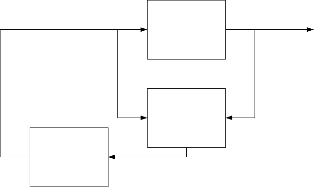
yu
CONTROLLED
SYSTEM
OBSERVER
- K
x
ˆ
Fig. 8.11. Block diagram of the closed-loop system with a state observer
Nowadays, theory of deterministic state observation is in mature state.
Fig. 8.11 shows how the observed state ˆx(t) is used in automatic control.
Luenberger introduced a concept of an observer illustrated in scheme in
Fig. 8.12. The observer has the form of the estimated linear process extended
with a feedback
u
L
(t)=L [y(t) − ˆy(t)] (8.210)
This is a proportional feedback loop designed to minimise the difference (y(t)−
ˆy(t)). The task of constructing a desired observer is thus transformed into the
problem of finding a suitable L.
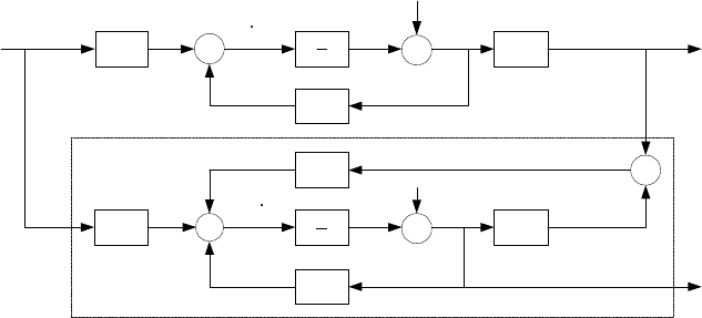
336 8 Optimal Process Control
u
s
1
s
1
x
0
x
x
y
0
x
ˆ
x
ˆ
x
ˆ
L
u
State observer
-
C
C
B
B
A
A
L
Fig. 8.12. Scheme of an observer
The observer will be designed for an observed system
˙x(t)=Ax(t)+Bu(t), x(0) = x
0
(8.211)
y(t)=Cx(t) (8.212)
The observer from Fig. 8.12 is described by equations
˙
ˆx(t)=Aˆx(t)+Bu(t)+L [y(t) − ˆy(t)] , ˆx(0) = ˆx
0
(8.213)
ˆy(t)=C ˆx(t) (8.214)
Let us now find a matrix L such that the estimation error
e(t)=x(t) − ˆx(t) (8.215)
with initial value
e(0) = x
0
− ˆx
0
(8.216)
converges asymptotically to zero.
From (8.215) follows
˙e(t)= ˙x(t) −
˙
ˆx(t) (8.217)
Substituting ˙x and
˙
ˆx form (8.211) and (8.213) yields
˙e(t)=Ax(t) − Aˆx(t) −L [y(t) − ˆy(t)] (8.218)
Finally, using (8.212) and (8.214) gives
˙e(t)=(A − LC) e(t), e(0) = e
0
(8.219)
The system (8.219) meets the requirements on observer design if it is asymp-
totically stable.
Asymptotic stability of the system (8.219) can be guaranteed for arbitrary
initial conditions of the observed system and the observer if and only if eigen-
values of the matrix (A − LC) lie in the left half-plane. Thus, matrix L has
to be chosen in such a way that the matrix (A −LC) be stable.

8.5 Observers and State Estimation 337
8.5.2 Kalman Filter
The Kalman filter is a special case of the Luenberger observer that is optimised
for the observation and input noises. We consider an optimal state estimation
of a linear system
˙x(t)=Ax(t)+ξ
x
(t) (8.220)
where ξ
x
(t)isn-dimensional stochastic process vector. We assume that the
processes have properties of a Gaussian noise
E {ξ
x
(t)} = 0 (8.221)
Cov (ξ
x
(t), ξ
x
(τ)) = E
ξ
x
(t)ξ
T
x
(τ)
= V δ(t −τ) (8.222)
Initial condition is given as
x(0) = ¯x
0
+ ξ
x0
(8.223)
where
E {x(0)} = ¯x
0
(8.224)
Cov (x(0)) = E
[¯x
0
− x(0)] [¯x
0
− x(0)]
T
= N
0
(8.225)
The mathematical model of the measurement process is of the form
y(t)=Cx(t)+ξ(t) (8.226)
where
E {ξ(t)} = 0 (8.227)
Cov (ξ(t), ξ(τ)) = E
ξ(t)ξ
T
(τ)
= Sδ(t − τ ) (8.228)
ξ
0
(t)andξ(t) are uncorrelated in time and with the initial state.
The problem is now to find a state estimate so that the cost function
I =
1
2
[x(0) − ¯x
0
]
T
N
−1
0
[x(0) − ¯x
0
]
+
1
2
t
f
0
[ ˙x(t) − Ax(t)]
T
V
−1
[ ˙x(t) − Ax(t)]
dt
+
1
2
t
f
0
[y(t) −Cx(t)]
T
S
−1
[y(t) −Cx(t)]
dt (8.229)
is minimised. The first right-hand term in (8.229) minimises the squared es-
timation error in initial conditions. The second term minimises the integral
containing squared model error. Finally, the third term penalises the squared
measurement error.
Let us define a fictitious control vector
u(t)= ˙x(t) − Ax(t) (8.230)

338 8 Optimal Process Control
The cost function I is then of the form
I =
1
2
[x(0) − ¯x
0
]
T
N
−1
0
[x(0) − ¯x
0
]
+
1
2
t
f
0
u
T
(t)V
−1
u(t)
+[y(t) −Cx(t)]
T
S
−1
[y(t) −Cx(t)] dt
(8.231)
and the optimal state estimation problem is then transformed into the deter-
ministic LQ control problem. The aim of this deterministic optimal control
is to find the control u(t) that minimises I of the form (8.231) subject to
constraint
˙x = Ax + u (8.232)
Hamiltonian of this problem is defined as
H =
1
2
u
T
V
−1
u +(y − Cx)
T
S
−1
(y − Cx)
+ λ
T
(Ax + u) (8.233)
The adjoint vector λ(t) is given as
˙
λ = −
∂H
∂x
= C
T
S
−1
y − C
T
S
−1
Cx − A
T
λ (8.234)
Final state is not fixed and gives the terminal condition for the adjoint vector
λ(t
f
)=0 (8.235)
x(0) is free as well and thus
x(0) = ¯x
0
+ N
0
λ(0) (8.236)
Optimal control follows from the optimality condition
∂H
∂u
= 0 (8.237)
This gives
V
−1
u + λ = 0 (8.238)
u(t)=−Vλ(t) (8.239)
We note that our original problem is the state estimation of the system with
random signals. This problem is commonly denoted as filtration and belongs to
a broader class of interpolation, filtration, and prediction. All three problems
are closely tied together and the same mathematical apparatus can be used
8.5 Observers and State Estimation 339
to solve each of them. In the sequel only the filtration problem in the Kalman
sense will be investigated.
Filtration can be thought of as the state estimation at time t
where all
information up to time t
is used.
Let ˆx (t|t
f
) be the optimal estimate at time t
f
with known data y(t)up
to time t
f
. The optimal estimate can be determined as
˙
ˆx (t|t
f
)=Aˆx (t|t
f
) −Vλ(t) (8.240)
Let us introduce a transformation
ˆx (t|t
f
)=z(t) − N (t)λ(t) (8.241)
The problem of finding the optimal state estimate can be solved if z(t)and
N(t) will be found. Equation (8.240) can be rewritten using the transforma-
tion (8.241) as
˙z(t) −
˙
N(t)λ(t) − N(t)
˙
λ(t)=A [z(t) − N(t)λ(t)] −Vλ(t) (8.242)
Substituting
˙
λ(t) from (8.234) and using (8.241) gives
˙z(t) −
˙
N(t)λ(t)
− N(t)
C
T
S
−1
y(t) −CS
−1
C (z(t) −N (t)λ(t)) −A
T
λ(t)
= A [z(t) −N (t)λ(t)] − Vλ(t) (8.243)
and after some manipulations
˙z(t) − N(t)C
T
S
−1
(y(t) −Cz(t)) − Az(t)
=
˙
N(t) − N(t)A
T
− AN(t)+N (t)CS
−1
CN(t) − V
λ(t) (8.244)
We can choose z(t)andN (t) such that
˙z(t)=Az(t)+N (t)C
T
S
−1
[y(t) −Cz(t)] (8.245)
z(0) = ¯x
0
(8.246)
V =
˙
N(t) − N(t)A
T
− AN(t)+N (t)CS
−1
CN(t) (8.247)
N(0) = N
0
(8.248)
Note that both equations (8.245) and (8.247) are solved forward in time from
t =0.
The state estimate ˆx (t
f
|t
f
) is based on available information up to time
t
f
.Ift = t
f
, the transformation (8.241) is given as
ˆx (t
f
|t
f
)=z(t
f
) −N (t
f
)λ(t
f
) (8.249)
Using (8.235) gives

340 8 Optimal Process Control
ˆx (t
f
|t
f
)=z(t
f
) (8.250)
State estimates are thus given continuously at time t as
ˆx (t|t)=Aˆx (t|t)+N (t)C
T
S
−1
[y(t) −C ˆx (t|t)] (8.251)
ˆx(0) = ¯x
0
(8.252)
where N(t) is solution of (8.247). Equations (8.251) and (8.247) describe the
Kalman filter.
Its gain is given for steady-state solution of (8.247) as
L = NC
T
S
−1
(8.253)
Define the estimation error
e(t)=x(t) − ˆx (t|t) (8.254)
then we can write
˙e(t)=
A −N (t)C
T
S
−1
C
e(t)+ξ
x
(t) −N (t)C
T
S
−1
ξ(t) (8.255)
where
e(0) = ξ
x0
(8.256)
From (8.255) and (8.256) follows
d
dt
(E {e(t)})=
A −NC
T
S
−1
C
E {e(t)},E{e(0)} = 0 (8.257)
Equation (8.257) gives
E {e(t)} = 0 (8.258)
and thus the estimate is unbiased. It can be shown that the covariance matrix
of the estimate is
Cov (e(t)) = N(t) (8.259)
The covariance matrix N is symmetric and positive semidefinite and it is a
solution of the Riccati equation similar to the LQ Riccati equation.
8.6 Analysis of State Feedback with Observer
and Polynomial Pole Placement
8.6.1 Properties of State Feedback with Observer
We have seen in previous chapters that the optimal LQ control design leads
to state feedback