Mikles J., Fikar M. Process Modelling, Identification, and Control

Подождите немного. Документ загружается.

8.6 Analysis of State Feedback with Observer and Polynomial Pole Placement 351

We choose the closed-loop characteristic polynomial as

o(s)f(s)=(s + 2)(s + 4)(s + 5)(s +6)

Our aim is to ﬁnd the transfer function of a controller that places the

closed-loop poles to locations speciﬁed by zeros of o(s)f(s). This transfer

function is of the form

R(s)=

s + q

+ p

s + p

and the coeﬃcients p

, p

, q

can be found as the solution of

equation



+5s +6



+ p

s + p



+(s+6)(q

s+q

)=(s+2)(s+4)(s+5)(s+6)

Equating coeﬃcients at either side of this equation gives ﬁve equations

with ﬁve unknowns

: p

:5p

+ p

=17

:6p

+5p

+ p

+ q

= 104

s :6p

+5p

+6q

+ q

= 268

:6p

+6q

= 240

The controller polynomials are then given as

p(s)=s

+12s +36

q(s)=2s +4

The derivation of the controller shows that pole placement as the only per-

formance criterium need not be satisfactory. For example, as the controller

does not contain integral part, the steady-state control error is non-zero –

if unit step change of the setpoint is assumed then is settles at the value

of 0.25.

The state feedback with observer interpreted using the input-output mod-

els naturally leads to the problem of the polynomial pole placement.

Calculation of o(s)andf(s) from (8.309), (8.331) is frequently not nec-

essary as the closed-loop poles can directly be assigned by the choice of a

polynomial c(s) on the right-hand side of the equation

a(s)p(s)+b(s)q(s)=c(s) (8.340)

Similarly, polynomials a(s), b(s) are often known and it is not necessary to

solve equation (8.296). Equation (8.340) plays a fundamental role in polyno-

mial pole placement.

8.6.3 Diophantine Equations

A scalar linear polynomial equation

352 8 Optimal Process Control

a(s)x(s)+b(s)y(s)=c(s) (8.341)

is called the Diophantine equation – after the mathematician Diophantos from

Alexandria (275 a. d.).

Polynomials a(s), b(s), and c(s) are given and polynomials x(s), y(s)are

unknown. The solvability of a Diophantine equation is characterised by the

next theorem.

Theorem 8.4 (Solvability of Diophantine equations). Let a(s), b(s),

c(s) be real valued polynomials. Equation (8.341) has a solution if and only if

the greatest common divisor of a(s), b(s) divides c(s).

It follows from the theorem that if a(s)andb(s) are coprime then the

Diophantine equation is solvable for any c(s) including c(s)=1.

If Diophantine equation is solvable then it has inﬁnitely many solutions.

If x



(s), y



(s) denote a particular solution then general solution can be

parametrised as

x(s)=x



(s)+

b(s)t(s) (8.342)

y(s)=y



(s) −¯a(s)t(s) (8.343)

where t(s) is an arbitrary polynomial, ¯a(s),

b(s) are coprime and

b(s)

¯a(s)

b(s)

a(s)

(8.344)

If a(s), b(s) are coprime then ¯a(s)=a(s),

b(s)=b(s).

Corollary: Among all solutions of the Diophantine equation there is one

x(s), y(s) where

deg x(s) < deg

b(s) (8.345)

Similarly, there exists unique solution of the same Diophantine equation where

deg y(s) < deg ¯a(s) (8.346)

Both solutions coincide if

deg a(s) + deg b(s) ≥ deg c(s) (8.347)

If equation (8.347) holds then the Diophantine equation has the minimum

degree solution and

deg x(s) = deg y(s) (8.348)

If equation (8.347) does not hold, there are solutions for minimal degree of

x(s) or for minimal degree of y(s).

8.6 Analysis of State Feedback with Observer and Polynomial Pole Placement 353

A versatile tool for Diophantine equations is Polynomial Toolbox for MAT-

LAB. Its use will be illustrated on examples.

Example 8.5:

www

Consider polynomials (see Example 8.4) a(s)=s

+5s +6, b(s)=s +6.

Find polynomials x(s), y(s) satisfying equation

a(s)x(s)+b(s)y(s)=c(s)

for various choices of polynomial c(s). Polynomial Toolbox for MATLAB

will be used – function [x,y]=axbyc(a,b,c) where the function argu-

ments are the same as our polynomials.

Case: c(s)=1+s. Entering the following commands in MATLAB

>> a = 6 + 5*s+s^2;

>> b = 6 + s;

>> [x, y] = axbyc(a, b, 1+s)

gives the solution:

x = -0.42

y = 0.58 + 0.42 s

Case: c(s)=(1+s)

>> [x, y] = axbyc(a, b, (1+s)^2)

x = 2.1

y = 1.9 - 1.1 s

Case: c(s)=(1+s)

(note: inequality (8.347) holds)

>> [x, y] = axbyc(a, b, (1+s)^3)

x = -4.4 + s

y = 4.6 + 2.4 s

Case: c(s)=(1+s)

(note: inequality (8.347) does not hold)

>> [x1, y1] = axbyc(a, b, (1+s)^4)

x1 = 1.3 - 2.5 s + s^2

y1 = -1.2 + 2.2 s + 1.5 s^2

This is minimum degree solution where deg(x

) = deg(y

)=2.

Case: c(s)=(1+s)

. Minimise the degree of polynomial x.

>> [x2, y2] = axbyc(a, b, (1+s)^4, ’minx’)

x2 = 52

y2 = -52 - 34s - 2 s^2 + s^3

Case: c(s)=(1+s)

. Minimise the degree of polynomial y.

>> [x2, y2] = axbyc(a, b, (1+s)^4, ’miny’)

x2 = 10 - s + s^2

y2 = -9.9 - 5.1s

Case: c =1+s. General solution of the form x(s)+f (s)t(s), y(s)+g(s)t(s)

is calculated where t(s) is arbitrary polynomial.

>> [x,y,f,g] = axbyc(a, b, 1+s)

x = -0.42

y = 0.58 + 0.42s

f = -0.6 - 0.1s

354 8 Optimal Process Control

g = 0.6 + 0.5s + 0.1 s^2

8.6.4 Polynomial Pole Placement Control Design

This control design is closely related to the solution of the Diophantine equa-

tion (8.340).

Consider the feedback system shown in Fig. 8.19. The process transfer

function is of the form

G(s)=

b(s)

a(s)

(8.349)

where polynomials

a(s)=a

+ a

n−1

+ ... + a

(8.350)

b(s)=b

n−1

+ b

n−2

+ ... + b

(8.351)

are coprime and the system is strictly proper.

The controller transfer function is

R(s)=

q(s)

p(s)

(8.352)

where

p(s)=p

+ p

−1

+ ... + p

(8.353)

q(s)=q

+ q

−1

+ ... + q

(8.354)

Desired stable characteristic polynomial of the closed-loop system is speciﬁed

c(s)=c

+ c

−1

+ ... + c

(8.355)

PP controller, case 1: Let c(s) be an arbitrary polynomial of degree n

2n − 1. Then there are polynomials p(s) of degree n

= n − 1andq(s)of

degree n

= n −1 such that

a(s)p(s)+b(s)q(s)=c(s) (8.356)

holds (see Example 8.5 – case 3). Controller R(s) is proper.

PP controller, case 2: Let c(s) be an arbitrary polynomial of degree n

=2n.

Then there are polynomials p(s) of degree n

= n and q(s) of degree

= n − 1 such that equation (8.356) holds (see Example 8.5 – case 6).

Controller R(s) is strictly proper.

We note that the choice of the polynomial degrees is not arbitrary. The

simplest controller is that with minimum degree of q(s). From the Diophantine

equation (8.356) follows that the minimum degree of q(s) is less than the

degree of a(s), thus n

= n − 1. The degree of the polynomial p(s) is them

given from realisability of the controller. Its degree has to be equal (PP 1)

or larger (PP 2) than the degree of q(s). Finally, the degree of c(s)canbe

determined from the degree of the left hand side of (8.356).

8.6 Analysis of State Feedback with Observer and Polynomial Pole Placement 355

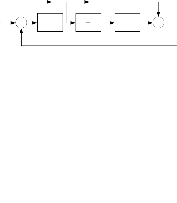
8.6.5 Integrating Behaviour of Controller

The closed-loop system consisting of the controlled system (8.296) and con-

troller (8.334) calculated from (8.295) cannot guarantee the zero steady-state

control error. As we have seen in previous chapters, to solve this issue, pure

integrator is needed in the controller as in Fig. 8.20.

()

Fig. 8.20. Closed-loop system with a pure integrator

The controller formed by the blocks q(s)/p(s) and 1/s assures that for step

changes of the setpoint variable w and step changes of disturbance d approach

the control error e and variable ˜u in the loop in Fig. 8.20 asymptotically zero

if q(s)andp(s) are solution of the equation

a(s)sp(s)+b(s)q(s)=c(s) (8.357)

and c(s) is a stable polynomial.

This can easily be proved using transfer functions between inputs w, d and

outputs e,˜u of the closed-loop in Fig. 8.20. These are of the form

(s)=

a(s)sp(s)

a(s)sp(s)+b(s)q(s)

(8.358)

(s)=

−a(s)sp(s)

a(s)sp(s)+b(s)q(s)

(8.359)

˜uw

(s)=

a(s)sq(s)

a(s)sp(s)+b(s)q(s)

(8.360)

˜ud

(s)=

−a(s)sq(s)

a(s)sp(s)+b(s)q(s)

(8.361)

Closed-loop poles are characterised by the polynomial a(s)sp(s)+b(s)q(s),

hence c(s) must be stable polynomial.

If w(t)=1(t) then the ﬁnal value theorem gives

lim

t→∞

e(t) = lim

t→∞

˜u(t) = 0 (8.362)

Equation (8.362) also holds for d(t)=1(t). This proves asymptotic properties

of the pole placement controller with integrator.

356 8 Optimal Process Control

The design procedure of the controller with integral action is as follows.

First the controlled system is formally modiﬁed to contain a pure integrator.

Polynomials p(s), q(s) are calculated from the Diophantine equation

˜a(s)p(s)+b(s)q(s)=c(s) (8.363)

where

˜a(s)=sa(s) (8.364)

with degree n

= n +1.

In the second step after polynomials p(s), q(s) are found from (8.363) the

integrator is moved to the controller. The controller transfer function is then

given as

R(s)=

q(s)

˜p(s)

(8.365)

where

˜p(s)=sp(s) (8.366)

PP controller with integral action, case 1: Let c(s) be an arbitrary polyno-

mial of degree 2n. Then there are polynomials p(s) of degree n

= n − 1

and q(s) of degree n

= n such that equation (8.363) holds. The controller

transfer function q(s)/p(s) is not proper. However, the real controller is

proper.

PP controller with integral action, case 2: Let c(s) be an arbitrary polyno-

mial of degree n

=2n

− 1=2n + 1. Then there are polynomials p(s)

of degree n

= n

− 1=n and q(s) of degree n

= n

− 1=n such

that equation (8.363) holds. The controller transfer function q(s)/p(s)is

proper. The real controller corresponds to the transfer function (8.365)

and is strictly proper.

PP controller with integral action, case 3: Let c(s) be an arbitrary polyno-

mial of degree n

=2n

=2(n + 1). Then there are polynomials p(s)

of degree n

= n

= n +1 and q(s) of degree n

= n

− 1=n such

that equation (8.363) holds. The controller transfer function q(s)/p(s)is

strictly proper.

We note again that the choice of the polynomial degrees is not arbitrary

and follows from the requirement that the controller numerator degree q(s)

should be minimal. In this case it is given by the Diophantine equation (8.363)

as n

= n. The controller cases then follow from the fact that the minimum

realisable degree of the controller denominator sp(s) is equal to the numerator

degree. Finally, when the degrees of p(s),q(s) are known, the degree of the

right hand side polynomial c(s) can de determined from the left hand side

polynomial of (8.363). The degree of c(s) can also be larger than 2n

. However,

8.6 Analysis of State Feedback with Observer and Polynomial Pole Placement 357

such controller would be too complicated. In practice, the controller degrees

are usually derived from cases 1 and 2.

Example 8.6:

www

The model of the controlled process is of the form

G(s)=

b(s)

a(s)

,a(s)=s +2,b(s)=1

The desired controller transfer function is given as

R(s)=

q(s)

sp(s)

where polynomials p(s), q(s) are solution of the equation

a(s)sp(s)+b(s)q(s)=c(s)

for various cases of the polynomial c(s). We use Polynomial Toolbox for

MATLAB.

Case: c(s)=(s +3)

. Typing in MATLAB Command Window

>> ai = s * (s+2);

>>b=1;

>> c = (s+3)^2;

>> [p,q] = axbyc(ai,b,c)

gives

p=1

q = 9+4s

The pole placement controller with integral action is of the form

R(s)=

4s +9

=4+

Case: c(s)=(s +3)

(s + 4).

>> ai = s * (s+2);

>>b=1;

>> c = (s+4) * (s+3)^2;

>> [p,q] = axbyc(ai,b,c)

yields

p = 8+s

q = 36+17s

The controller with integral action is of the form

R(s)=

17s +36

s (s +8)



17 +



s +8



Case: c(s)=(s +3)

(s +4)

358 8 Optimal Process Control

>> ai = s * (s+2);

>>b=1;

>> c = (s+3)^2 * (s+4)^2;

>> [p,q] = axbyc(ai,b,c)

Result:

p = 64+12s+s^2

q = 140+40s-15 s^2

The controller with integral action is of the form

R(s)=

−15s

+40s + 140

s (s

+12s + 64)

Example 8.7:www

The model of the controlled process is of the form

G(s)=

b(s)

a(s)

,a(s)=s

+4s +4,b(s)=s +1

The task is to design a controller in the same way as in Example 8.6.

Case: c(s)=(s +3)

. Typing in MATLAB Command Window

>> ai = s * (s^2+4s+4);

>> b = s+1;

>> c = (s+3)^4;

>> [p,q] = axbyc(ai,b,c)

gives

p = -15+s

q = 81+87s+23 s^2

The pole placement controller with integral action is of the form

R(s)=

23s

+87s +81

s (s −15)

s −15



87 +

+23s



Case: c(s)=(s +3)

>> ai = s * (s^2+4s+4);

>> b = s+1;

>> c = (s+3)^5;

>> [p,q] = axbyc(ai,b,c)

yields

p = -22+11s+ s^2

q = 240+250s+64s^2

The controller with integral action is of the form

R(s)=

64s

+ 250s + 240

s (s

+11s −22)

+11s −22



250 +

240

+64s



We can see that the controller denominator polynomial p(s) is unstable.

However, if the roots of the polynomial c(s) have been changed from −3

to −1.5, the denominator would have been stable.

8.6 Analysis of State Feedback with Observer and Polynomial Pole Placement 359

Even if an unstable controller is capable to guarantee stable closed-loop,

from practical point of view it is more suitable to have a stable controller.

In general, stability of p(s) is inﬂuenced by its coeﬃcients that are deter-

mined from from the closed-loop roots. Therefore, placement of the poles

for strong stability is not trivial.

Example 8.6 shows that the pole placement method can be used for design

of PI and PID controllers.

PI Controller for the First Order System

Consider the controlled process model described by the ﬁrst order transfer

function. If we choose the characteristic polynomial of the closed-loop systems

c(s) to be of the second degree then the structure of the pole placement

controller is with the transfer function (see Example 8.6 – case 1)

R(s)=

s + q

(8.367)

This transfer function is equivalent to the structure of the PI controller

(s)=K

(8.368)

where

= q

(8.369)

This controller was also derived in Chapter 7.4.6 (see page 285).

PI Controller with a Filter for the First Order System

Consider the controlled process model described by the ﬁrst order transfer

function. If we choose the characteristic polynomial of the closed-loop sys-

tems c(s) to be of the third degree then the structure of the pole placement

controller is with the transfer function (see Example 8.6 – case 2)

R(s)=

s + q

s (s + p

)

(8.370)

This transfer function is equivalent to the structure of the PI controller with

a ﬁrst order ﬁlter

PIF

(s)=





PIF

s +1



(8.371)

where

PIF

(8.372)

360 8 Optimal Process Control

PID Controller for the Second Order System

Consider the controlled process model described by a strictly proper second

order system. If we choose the characteristic polynomial of the closed-loop

systems c(s) to be of the fourth degree then the structure of the pole placement

controller is with the transfer function (see Example 8.7 – case 1)

R(s)=

+ q

s + q

s (s + p

)

(8.373)

This transfer function is equivalent to the structure of the PID controller

PIDF

(s)=



+ T



PIDF

s +1



(8.374)

where

PIDF

(8.375)

The transfer function (8.373) also corresponds to the PID controller with

derivative action ﬁltered by the ﬁrst order ﬁlter

PIDZ

(s)=Z

PIDZ

s +1

(8.376)

where

− q

− p

+ q

PIDZ

(8.377)

PID Controller with a Filter for the Second Order System

Consider the controlled process model described by a strictly proper second

order system. If we choose the characteristic polynomial of the closed-loop

systems c(s) to be of the ﬁfth degree then the structure of the pole placement

controller is with the transfer function (see Example 8.7 – case 2)

R(s)=

+ q

s + q

s (s

+ p

s + p

)

(8.378)

This transfer function is equivalent to the structure of the PID controller with

a ﬁlter

PIDF2

(s)=



+ T



F 2

+ p

F 1

s +1



(8.379)

where

F 2

F 1

(8.380)