Mattingly J.D., Heiser W.H., Pratt D.T. Aircraft Engine Design

Подождите немного. Документ загружается.

256 AIRCRAFT ENGINE DESIGN

where the subscripts i and e correspond to the inlet and exit, respectively. The

diffusion factor is an analytical expression directly related to the size of the adverse

pressure gradient to be encountered by the boundary layer on the suction surface

of the cascade airfoil. It is therefore a measure of the danger of boundary layer

separation and unacceptable losses or flow instability. The two terms of Eq. (8.1)

clearly embody the physics of the situation, the first representing the average static

pressure rise in the airfoil channel and the second the additional static pressure

rise along the suction surface due to curvature or lift.

The goal of the designer is to be able to maintain high aerodynamic efficiency at

large values of D because that allows the number of stages (that is, lower

Ve/Vi)

and/or airfoils (that is, lower a) to be reduced. Thus, the ability to successfully

design for large values of D is a sign of technological advancement and the basis

for superior compressors. Even in this world of sophisticated computation, fan and

compressor designers use the diffusion factor almost universally as the measuring

rod of technological capability. Any reasonably competent contemporary organi-

zation is able to cope with values of D up to 0.5. Values of D up to 0.6 are possible

if you can count on state-of-the-art aerodynamic understanding and design tools,

and extensive development testing.

A final note of interest about the diffusion factor is that it is based on the flow

geometry alone and is therefore silent about the geometrical details of the airfoil

itself. This provides a great convenience that makes much analytical progress

possible. In fact, what is unique about the approach employed here is that the

diffusion factor equation is used as a constraining relationship from the start,

rather than as a feasibility check at the end.

Assumptions

1) Repeating row/repeating airfoil cascade geometry (oq = fie = a3, fll = or2 =

33).

2) Two-dimensional flow (that is, no property variation or velocity component

normal to the flow).

3) Constant axial velocity (ul = u2 = u3).

4) Stage polytropic efficiency ec represents stage losses.

5) Constant mean radius.

6) Calorically perfect gas with known Fc and Rc.

Analysis.

Please note that the assumption of constant axial velocity, which

is consistent with modern design practice, greatly simplifies the analysis because

every velocity triangle in Fig. 8.1 has the same base dimension.

Given:

D, MI, F, or, ec.

1) Conservation of mass:

rh = plUjA1 = p2u2A2 = p3u3A3

plAI = p2A2 = p3A3

2) Repeating row constraint:

Since 32 = oq, then

1)2R ~ U 1 ~ (.or -- 1) 2

(8.2)

(8.3)

DESIGN: ROTATING TURBOMACHINERY 257

Vl+1) 2 =wr

(8.4)

Incidentally, since f13 = 0/2, then

1)3R

= 1)2, and

I) 3 ~ 60r -- 1)3R ~ (.or -- 1)2

then by Eq. (8.3)

1)3 ~" 1)1

and the velocity conditions at the stage exit are indeed identical to those at the

stage entrance, as shown in Fig. 8.1.

3) Diffusion factor (D):

Since both

(V2R)+1)IR--1)2R

D = 1- V1R 2aVIR

and

V3 ) I)2 -- 1)3

_ 1-E + - g-vS

= (tan ot 2

tan ~1

o coso, ÷ )coso

COS Ol 1 / k 20"

(8.5)

20" + sinoq

I" -- (8.7)

COS Ot 1

In words, Eq. (8.6-7) shows that there is only

one

value of or2 that corresponds to

the chosen values of D and 0" for each al. Thus, the entire flowfield geometry is

dictated by those choices.

4) Degree of reaction (°Rc):

Another common sense measure of good compressor stage design is the degree

of reaction

rotor static temperature rise T2 - T1

°Re = stage static temperature rise- T3- T1 (8.8)

For a perfect gas with

p ~ constant,

°Rc-- T2-T1

~ [P2- P________~I] (8.9)

T3 - Tl L P3 - P1 .J p~const

In the general case it is desirable to have

°Rc

in the vicinity of 0.5 because the

stator and rotor rows will then "share the burden" of the stage static temperature

where

20-(1 - D)F + ~/1 -'2 + 1 - 4o'2(1 - D) 2

(8.6)

cos or2 = I "2 + 1

are the same for both the stator and rotor airfoil cascades, they need be evaluated

only once for the entire stage. Rearranging Eq. (8.5) to solve for or2, it is found that

258 AIRCRAFT ENGINE DESIGN

rise, and neither will benefit at the expense of the other. This is another way of

avoiding excessively large values of D.

A special and valuable characteristic of repeating stage, repeating row compres-

sor stages is that °Re must be exactly 0.5 because of the forced similarity of the

rotor and stator velocity triangles. You can confirm this by inspecting Eq. (8.8)

and recognizing that the kinetic energy drop and hence the static temperature rise

are the same in the rotor and stator.

5) Stage total temperature increase

(ATt)

and ratio

(Tt3/Ttl):

From the Euler pump and turbine equation with constant radius

(.or

ht3 - htt

= --(v2

Vl)

which, for a calorically perfect gas, becomes

o)r

cp(Tt3 --

Ttl)

= --(112 -- Vl) (8.10)

whence, using Eq. (8.4)

Thus

cpCTt3 --

rtl) = --(v2 "t- Vl)(V2 -- Vl) --

(v+- Vl _ (v#- v?)

gc gc

ATr = Zt3_ Ztl _ V2- V? _ V?

(c0s20/1 )

Cpgc Cpgc ~, cos

20/2 1

AT t

COS 2 o/1

-- -- -- 1 (8.11)

Vl2/cpgc

cos 20/2

Since V 2 =

M2yRgcT

and Tt = T[1 + (y - 1)M2/2], then the stage temperature

ratio is given by

Tt3 (y - 1)Mi 2

(COS2 0/1

)

rs -- Ttl -- 1 -~(-y

--- 1-~12/2

I,,C--~S2~2 l + 1 (8.12)

This relationship reveals that, for a given flow geometry, the stage total temperature

rise is proportional to Ttl and M12.

6) Stage pressure ratio:

From Eq. (4.9b-CPG)

Pt3 _ ( Tt3 ~ yec/(y-1)

Zrs - ~ \ r. / =

(Ts) Yec/(Y-l)

(8.13)

7) Stage efficiency:

From Eq. (4.9b-CPG)

Tt3i

-- Ztl

7l" (g-1)/F -- 1 r e`.- 1

Us -- -- -- -- (8.14)

Zt3

Ttl T s -- 1 rs -- 1

DESIGN: ROTATING TURBOMACHINERY 259

8) Stage exit Mach number:

Since V3 = V1 and V 2 =

M2yRgcT,

then

M3 _ ~T~ ~ 1

Mll -- = rs[1 + (?/- 1)M2/2] - ()' - 1)M2/2 -< 1 (8.15)

Since

T3/T1

> 1, then

M3/M1

< 1, and the Mach number gradually de-

creases as the flow progresses through the compressor, causing compressibility

effects to become less important.

9) Wheel speed/inlet velocity ratio

(cor/V1):

One of the most important trigonometric relationships is that between the mean

wheel speed (wr) and the total cascade entrance velocity (V1) because the latter

is usually known and, as you shall find in Sec. 8.2.3, the former places demands

upon the materials and structures that can be difficult to meet.

Since

V1 = ul/cos0/l and ~or

= 1) 2 -t- 1)1 =

ul(tan0/l + tan0/2)

then

wr/V1

= cos0/1 (tan 0/1 + tan 0/2)

10) Inlet relative Mach number (M1R):

Since

(8.16)

then

1/1 = Mlal

= ul/cos0/l

and V1R = MIRa1

= Ul/COS0/2

M1R

COS 0/1

-- -- -- (8.17)

M1 cos 0/2

Since o~ 2 "> 0/1, then M1R > M1 and M1 must be chosen carefully in order to

avoid excessively high inlet relative Mach numbers.

General solution.

The behavior of every imaginable repeating row compressor

stage with given values of D, M1, y, ~, and ec can now be computed. This is done

by selecting any initial value for 0/1 and using the following sequence of equations

expressed as functional relationships:

0/2 =

f (D, cr,

0/1) (8.6)

A0/ ~ 0/2 -- 0/1

rs = f(M1, y, 0/1,0/2)

(8.12)

7rs = f(rs, y, ec)

(8.13)

or/V1

= f(0/1,0/2) (8.16)

MIR/M1

= f(0/1, 0/2) (8.17)

Note that only r, and Jr, depend upon M1 and that the process may be repeated to

cover the entire range of reasonable values of 0/1.

260 AIRCRAFT ENGINE DESIGN

2.4 80

2.2 70

2.0 60

O~ 2 (deg)

1.8 50

o~ r / V~

1.6 40

~'s

1.4 30

M~R/M~

1.2 20

Aa (deg)

1.0 10

0.8 0

0 10 20 30 40 50 60 70

a t (deg)

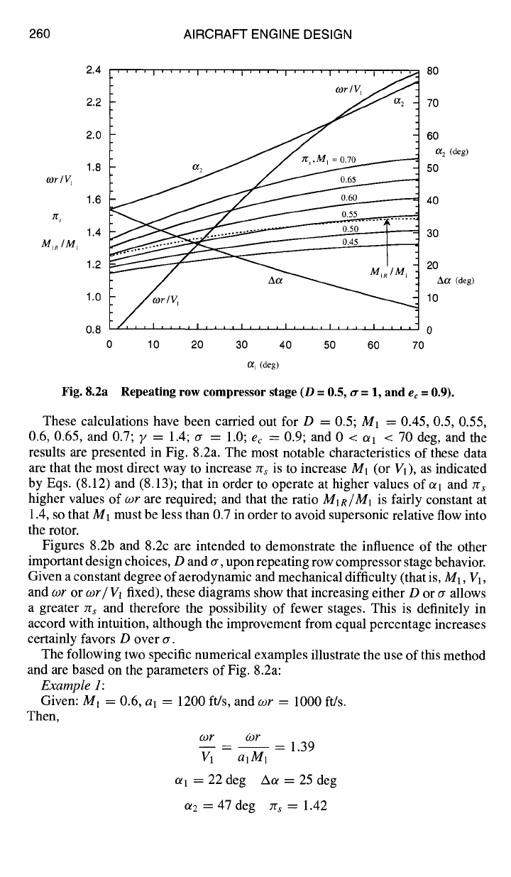
Fig. 8.2a Repeating row compressor stage (D = 0.5, ~r = 1, and

ec =

0.9).

These calculations have been carried out for D = 0.5; M1 = 0.45, 0.5, 0.55,

0.6, 0.65, and 0.7; g = 1.4; cr = 1.0; ec ---= 0.9; and 0 < oq < 70 deg, and the

results are presented in Fig. 8.2a. The most notable characteristics of these data

are that the most direct way to increase :rs is to increase M1 (or Vl), as indicated

by Eqs. (8.12) and (8.13); that in order to operate at higher values of Oil and Zrs

higher values of wr are required; and that the ratio M1R/M1 is fairly constant at

1.4, so that M1 must be less than 0.7 in order to avoid supersonic relative flow into

the rotor.

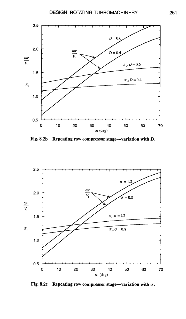
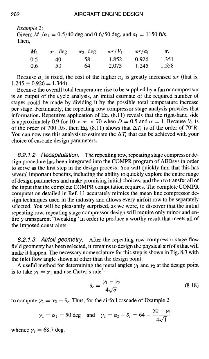
Figures 8.2b and 8.2c are intended to demonstrate the influence of the other

important design choices, D and or, upon repeating row compressor stage behavior.

Given a constant degree of aerodynamic and mechanical difficulty (that is, Mb V1,

and cor or cor/Vz fixed), these diagrams show that increasing either D or a allows

a greater zr, and therefore the possibility of fewer stages. This is definitely in

accord with intuition, although the improvement from equal percentage increases

certainly favors D over or.

The following two specific numerical examples illustrate the use of this method

and are based on the parameters of Fig. 8.2a:

Example 1:

Given: MI = 0.6, al ---- 1200 ft/s, and ~or --- 1000 ft/s.

Then,

(.or o)r

-- -- 1.39

V1 aiM1

cq =22deg Aol=25deg

ot2=47deg zr,= 1.42

DESIGN: ROTATING TURBOMACHINERY 261

0 10 20 30 40 50 60 70

a~ (deg)

Fig. 8.2b Repeating row compressor stage---variation with D.

(Dr

2.5

2.0

(Dr

1.5

7t" s

1.0

0.5

2.5

2.0

1.5

1.0

0.5

Fig. 8.2c

' ' ' ' I ' ' ' ' I ' ' ' ' I ' ' ' ' I ' ' ' ' I ' ' ' ' I ' ' ' '

~,,o- =1.2

~,ff =0.8

, , , I , , , , I , , , , I , , , I I I I I i [ a i i i I i i i i

10 20 30 40 50 60

a~ (deg)

Repeating row compressor stage--variation with tT.

262 AIRCRAFT ENGINE DESIGN

Example 2:

Given:Ml/al = 0.5/40 degand 0.6/50 deg, and al = 1150fffs.

Then,

~1,

deg u2, deg wr/Vl ~r/al Ks

0.5 40 58 1.852 0.926 1.351

0.6 50 64 2.075 1.245 1.558

Because al is fixed, the cost of the higher Zrs is greatly increased wr (that is,

1.245 - 0.926 = 1.344).

Because the overall total temperature rise to be supplied by a fan or compressor

is an output of the cycle analysis, an initial estimate of the required number of

stages could be made by dividing it by the possible total temperature increase

per stage. Fortunately, the repeating row compressor stage analysis provides that

information. Repetitive application of Eq. (8.11) reveals that the right-hand side

is approximately 0.9 for 10 < c~1 < 70 when D = 0.5 and tr = 1. Because V1 is

of the order of 700 ft/s, then Eq. (8.11) shows that ATt is of the order of 70°R.

You can now use this analysis to estimate the ATt that can be achieved with your

choice of cascade design parameters.

8.2.1.2 Recapitulation. The repeating row, repeating stage compressor de-

sign procedure has been integrated into the COMPR program of AEDsys in order

to serve as the first step in the design process. You will quickly find that this has

several important benefits, including the ability to quickly explore the entire range

of design parameters and make promising initial choices, and then to transfer all of

the input that the complete COMPR computation requires. The complete COMPR

computation detailed in Ref. 11 accurately mimics the mean line compressor de-

sign techniques used in the industry and allows every airfoil row to be separately

selected. You will be pleasantly surprised, as we were, to discover that the initial

repeating row, repeating stage compressor design will require only minor and en-

tirely transparent "tweaking" in order to produce a worthy result that meets all of

the imposed constraints.

8.2.1.3 Airfoil geometry.

After the repeating row compressor stage flow

field geometry has been selected, it remains to design the physical airfoils that will

make it happen. The necessary nomenclature for this step is shown in Fig. 8.3 with

the inlet flow angle shown at other than the design point.

A useful method for determining the metal angles Yl and Y2 at the design point

is to take Yl = oq and use Carter's rule 3,~1

~c -- ~/1 -- ~/2 (8.18)

to compute Y2 = 0/2

-- ~c"

Thus, for the airfoil cascade of Example 2

~=al=50deg

and V2 = 0/2 - ~c ~-- 64

50- )/2

whence y2=68.7 deg.

DESIGN: ROTATING TURBOMACHINERY 263

i_S

• X

- 7e

a i- O~ e = turning angle

7i - 7e

= airfoil camber angle

°~i- Yi-- incidence angle

ae - 7e

= & = exit deviation

tr = c/s

= solidity

O = stagger angle

Fig. 8.3

Cascade airfoil nomenclature.

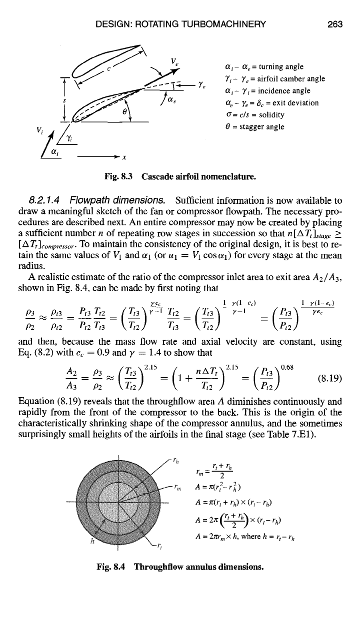
8.2.1.4 Flowpath dimensions.

Sufficient information is now available to

draw a meaningful sketch of the fan or compressor flowpath. The necessary pro-

cedures are described next. An entire compressor may now be created by placing

a sufficient number n of repeating row stages in succession so that

n[ATt]stage >_

[ATt]comp .......

TO maintain the consistency of the original design, it is best to re-

tain the same values of V1 and or1 (or Ul = VI cosotl) for every stage at the mean

radius.

A realistic estimate of the ratio of the compressor inlet area to exit area

A2/A3,

shown in Fig. 8.4, can be made by first noting that

yec

1--y(1--ec)

l--v(l--e,.)

p._~3 pt.~3 __ Pt3 Zt2 _ (Tt3~-~-I Tt2 (Zt3 ~ y-I : (Pt3X~ yec

P2 Pt2 -~t2 T-~t3 \ Tt2,/ ~t3 = \ ~t2 J ~, P,2 ]

and then, because the mass flow rate and axial velocity are constant, using

Eq. (8.2) with ec = 0.9 and y = 1.4 to show that

A2 P3 .~ (Tt3~ 2"15 (

nATt~215=

(Pt3~ 0"6s

~33

-- P~

\~t2,/

= 1 +

-~t2 ,/ \~,/

(8.19)

Equation (8.19) reveals that the throughflow area A diminishes continuously and

rapidly from the front of the compressor to the back. This is the origin of the

characteristically shrinking shape of the compressor annulus, and the sometimes

surprisingly small heights of the airfoils in the final stage (see Table 7.El).

Fig. 8.4

~,+rh

rm- 2

= 7C(r t + rh) x

(r t-

rh)

A = 2;c(~)X (rt-rh)

A = 2arr m x h, where h = r t-

r h

Throughflow annulus dimensions.

264

AIRCRAFT ENGINE DESIGN

l 2 3

hi+h2 c

rh Wr

= ~ (~-)~ cos gh

h2+h3 c

= T cos

o,,

Centerline

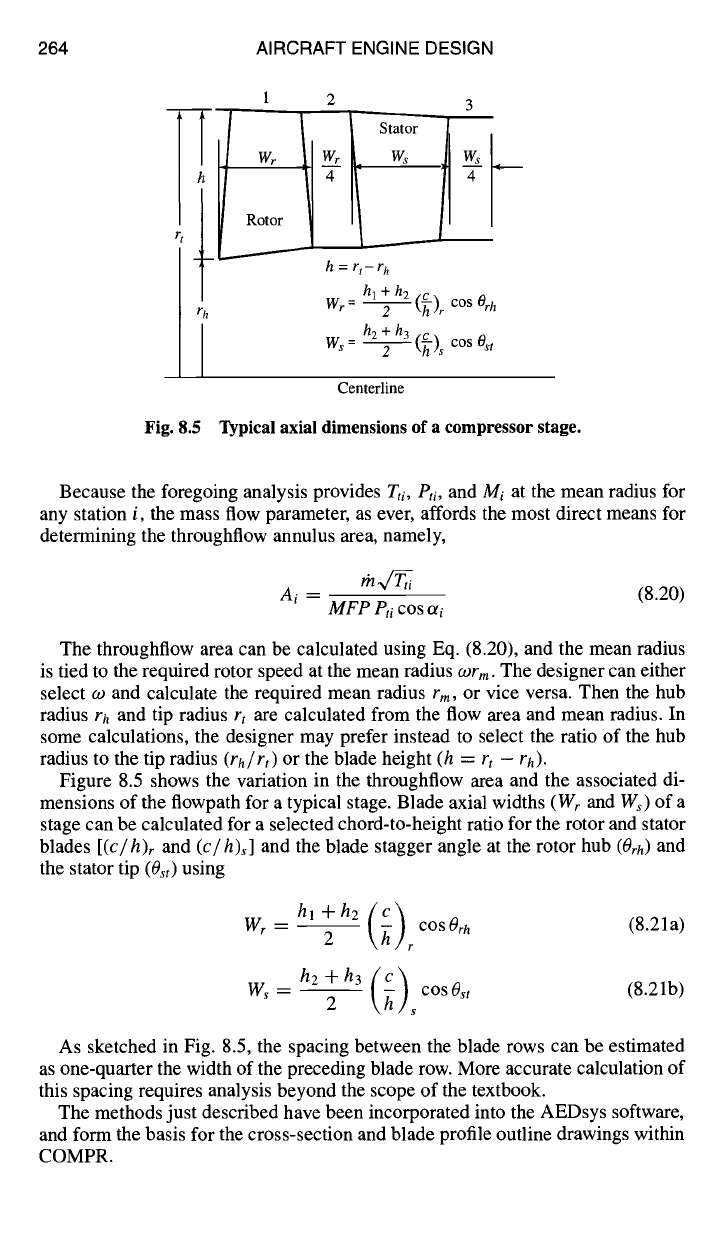
Fig. 8.5 Typical axial dimensions of a compressor stage.

Because the foregoing analysis provides

Tti , Pti,

and

at the mean radius for

any station i, the mass flow parameter, as ever, affords the most direct means for

determining the throughflow annulus area, namely,

Ai -- (8.20)

MFP

eti

COS o/i

The throughflow area can be calculated using Eq. (8.20), and the mean radius

is tied to the required rotor speed at the mean radius

COrm.

The designer can either

select CO and calculate the required mean radius

rm,

or vice versa. Then the hub

radius

and tip radius

rt are

calculated from the flow area and mean radius. In

some calculations, the designer may prefer instead to select the ratio of the hub

radius to the tip radius

(rh/rt)

or the blade height

(h = rt

- rh).

Figure 8.5 shows the variation in the throughflow area and the associated di-

mensions of the flowpath for a typical stage. Blade axial widths

(Wr and W~)

of a

stage can be calculated for a selected chord-to-height ratio for the rotor and stator

blades

[(c/h)r

and (c/h)s]

and the blade stagger angle at the rotor hub

(Orb)

and

the stator tip (0st) using

~ cos

Orb

(8.21a)

Ws-- h2+h3 (c)

2 ~ cos O~t (8.21b)

As sketched in Fig. 8.5, the spacing between the blade rows can be estimated

as one-quarter the width of the preceding blade row. More accurate calculation of

this spacing requires analysis beyond the scope of the textbook.

The methods just described have been incorporated into the AEDsys software,

and form the basis for the cross-section and blade profile outline drawings within

COMPR.

DESIGN: ROTATING TURBOMACHINERY 265

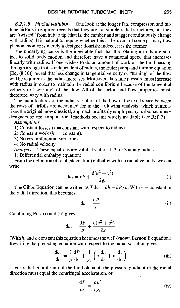
8.2. 1.5 Radial variation.

One look at the longer fan, compressor, and tur-

bine airfoils in engines reveals that they are not simple radial structures, but they

are "twisted" from hub to tip (that is, the camber and stagger continuously change

with radius). It is natural to inquire whether this is the result of some primary flow

phenomenon or is merely a designer flourish; indeed, it is the former.

The underlying cause is the inevitable fact that the rotating airfoils are sub-

ject to solid body motion and therefore have a rotational speed that increases

linearly with radius. If one wishes to do an amount of work on the fluid passing

through a stage that is independent of radius, the Euler pump and turbine equation

[Eq. (8.10)] reveal that less change in tangential velocity or "turning" of the flow

will be required as the radius increases. Moreover, the static pressure must increase

with radius in order to maintain the radial equilibrium because of the tangential

velocity or "swirling" of the flow. All of the airfoil and flow properties must,

therefore, vary with radius.

The main features of the radial variation of the flow in the axial space between

the rows of airfoils are accounted for in the following analysis, which summa-

rizes the original, now classical, approach profitably employed by turbomachinery

designers before computational methods became widely available (see Ref. 3).

Assumptions

1) Constant losses (s = constant with respect to radius).

2) Constant work

(hi =

constant).

3) No circumferential variations.

4) No radial velocity.

Analysis.

These equations are valid at station 1, 2, or 3 at any radius.

1) Differential enthalpy equation:

From the definition of total (stagnation) enthalpy with no radial velocity, we can

write

d(u 2 +

1) 2)

dht

= dh + (i)

2gc

The Gibbs Equation can be written as

Tds = dh - dP/p.

With s = constant in

the radial direction, this becomes

dh = -- (ii)

Combining Eqs. (i) and (ii) gives

dP d(u 2 + v 2)

dht = -- +

p 2gc

(With

ht and p

constant this equation becomes the well-known Bernoulli equation.)

Rewriting the preceding equation with respect to the radial variation gives

dht_ldP

1( du dr)

d---;- p dr + --gc u dr + v -&r

(iii)

For radial equilibrium of the fluid element, the pressure gradient in the radial

direction must equal the centrifugal acceleration, or

pv 2

- -- (iv)

dr r gc