Massoud M. Engineering Thermofluids: Thermodynamics, Fluid Mechanics, and Heat Transfer
Подождите немного. Документ загружается.


522 IVb. Heat Transfer: Forced Convection
Example IVb.2.1. Derive Equation IIIa.3.23-1 directly from an energy balance
written for a control volume.
Solution: The derivation is similar to heat conduction in a solid. However, while
solid is stationary, we know that there is fluid motion inside the boundary layer.
Hence, our derivation must take this into account. We begin by considering flow
into and out of an elemental control volume taken inside the boundary layer, as
shown in the figure. An energy balance for the elemental control volume takes the
form of:
q'''
.
Heat & Fluid
Flow Field
V
S
Net Flux of Energy
By Conduction
Net Flux of Energy
By Convection
Rate of Energy
Production
Rate of Change o
f
Internal Energy
+
=
We integrate the energy balance over the entire heat and fluid flow fields to ob-
tain:
()
()
V
V
VV
S
S
T
k T ndS Vh ndS q d c d
t
ρρ
´
´
´
µ
µ
µ
µ
µ
µ
¶
¶
¶
∂
−−∇⋅ − ⋅ + =′′′
³
∂
K
K
KK
We can convert the surface integrals to volume integrals by using Gauss’s theo-
rem, Equation VIIc.1.25:
0V
V
=
µ
¶
´
¸
¹
·
¨
©
§
′′′
+
∂
∂
−⋅∇−∇⋅∇ dq
t
T
cTVcTk
PP
K
K
K
ρρ
where we have assumed incompressible flow for which, dh = c
p
dT. For constant
k, we obtain:
()
0
2
=
∂
∂
−
′′′
+⋅∇+∇⋅−∇
t
T
cqVTTVcTk
pp
ρρ
K
K
K
K
For incompressible flow, the second term in the parentheses is zero (see Exam-
ple IIIa.3.3). Dividing by k and introducing thermal diffusivity (
p
ck
ρα
/= ), the
above equation reduces to:
2
1 T
Tq V T
t
α
∂
§·
′′′
∇+ = +⋅∇
¨¸
∂
©¹
KK
IIIa.3.23-2
Equation IIIa.3.23-2 reduces to Equation IVa.2.2 for stagnant fluid. Using the
substantial derivative D/DT, Equation IIIa.3.23-2 may also be written as:
2
1
D
T
Tq
D
t
α
′′′
∇+ =
IIIa.3.23-3

2. Analytical Solution 523
Equations IIIa.3.20-1 and IIIa.3.23-1 are second-order, coupled partial differen-
tial equations. Finding an analytical solution by integration is not an easy task.
However, in this case we know how the profiles of both variables look like.
Therefore, we try to solve these equations by guessing the functional relationship
for V
x
= f
1
(y) and T = f
2
(y). Since for each equation we have four boundary condi-
tions, two at the surface and two at the edge of boundary layer, we use a third or-
der polynomials. Thus, we express velocity as a function of y as:
3
4
2
321
ycycyccV
x
+++=
All we have to do now is to find the four unknown coefficients, c
1
through c
4
, so
that the above polynomial fits both Equation IIIa.3.20-1 and the specified sets of
boundary conditions. The sets of boundary conditions are:
at y = 0: V
x
= 0 and ∂
2
V
x
/∂y
2
= 0
at y =
δ: V
x
= V
f
and ∂V
x
/∂y = 0
Using conditions at y = 0, we find c
1
= c
3
= 0. We now use conditions at y = δ to
find c
2
and c
4
. From y = δ, V
x
= V
f
, we find c
2
δ + c
4
δ
3
= V
f
. From y = δ, ∂V
x
/∂y =
0, we find c
2
+ 3c
4
δ
2
= 0. Solving this set, we find c
2
and c
4
in terms of δ, V
x
, and
V
f
as c
2
= 3V
f
/2δ and c
4
= –V
x
/2δ
3
. Therefore, the velocity profile becomes:
3
į2
1
į2
3
¸
¹
·
¨
©
§
−=
yy
V
V
f
x
IVb.2.1
Due to the similarity of the governing Equations IIIa.3.20-1 and IIIa.3.23-1, we
expect that temperature can be described by a similar function:
3
į'2
1
į'2
3
¸
¹
·
¨
©
§
−=
−
−
yy
TT
TT
sf
s
IVb.2.2
Although we were able to find an analytical solution for these profiles, we are far
from declaring victory. This is because in Equation IVb.2.1, V
x
is expressed in
terms of the unknown
δ, yet to be determined. We did expect this additional twist,
as we used our engineering intuition and picked a profile. We then found the co-
efficients of the function representing the profile from the boundary conditions.
But we still have no guarantee that the chosen profile would satisfy the governing
equation itself. The thickness of the boundary layer,
δ, is indeed the final re-
quirement to ensure the chosen profile does satisfy the governing equation. We
should then embark on finding
δ. Similar to the profile for V
x
, we first guess a
profile for
δ and then try to find the related coefficient. However, the solution for
δ is not as straightforward as the solution we managed to find for the velocity pro-
file.
524 IVb. Heat Transfer: Forced Convection
Determination of the Hydrodynamic Boundary Layer Thickness
for Laminar Flow over Flat Plate
To find the thickness of the hydrodynamic boundary layer,
δ, we first note that δ
is only a function of x. To find this function, we resort to the conservation equa-
tion of mass, Equation IIIa.3.13-1:
0=
∂
∂
+
∂
∂
y
V
x
V
y
x
this equation can be approximated as V
f
/x + V
y
/δ = 0. Therefore V
y
is proportional
to V
y
∝ V
f
δ/x. We now apply the same approximation to the governing momen-
tum equation, Equation IIIa.3.20-1 while substituting for V
y
. This results in:
2
į
į
į
ff
f
f
f
V
v
V
x
V
x
V
V ≈+
from which δ is found to have a functional relationship as
f
Vvx /į ∝ .
Having obtained the shape of the function for
δ, we substitute it into Equa-
tion IIa.3.20-1, being a partial differential equation. Fortunately, we can convert
this equation to an ordinary differential equation by noticing that both V
x
and V
y
can be expressed in terms of a stream function ψ. That is to say that if V
x
= ∂ψ/∂y
and V
y
= –∂ψ/∂x then the continuity equation (Equation IIIa.3.13-1) is automati-
cally satisfied. To find the stream function, we integrate either of these relations
while noting from Equation IVb.2.1 that V
x
/V
f
= f(
β
) where
β
= y/δ. Hence
³
µ
¶
´
==
µ
µ
¶
´
µ
¶
´
=== )()()()(ȥ
ββββββ
F
V
vx
Vdf
V
vx
Vdf
V
vx
VdyfVdyV
f
f
f
f
f
ffx
Thus F(
β
) = ψ(x, y)/(vxV
f
)
1/2
. Having ψ and F(
β
), we find V
x
and V
y
:
V
x
= ∂ψ/∂y = (dF/d
β
)V
f
/2
V
y
= –∂ψ/∂x = [
β
F’(
β
) – F(
β
)](vV
f
/x)
1/2
/2
Having V
x
and V
y
, we can find other derivatives and substitute the results in Equa-
tion IIIa.3.20-1 to obtain:
02
2
2
3
3
=+
ββ
d
Fd
F
d
Fd
IVb.2.3
This equation is subject to three boundary conditions, two of which deal with y = 0
(i.e., V
x
(x, 0) = V
y
(x, 0) = 0). This is equivalent with F(
β
= 0) = dF(
β
= 0)/d
β
= 0.
The third boundary condition is at y =
∞, i.e., V
x
(x, ∞) = V
f
. This is equivalent
with dF(
∞)/d
β
= 1.
Blasius recommended the above method for solving Equation IVb.2.3. A strict
analytical solution has not been found for Equation IVb.2.3. Schlichting found a
2. Analytical Solution 525
τ
s
P
x
P
x + dx
T
f
δ
x
y
(V
x
)
f
x
o
δ'
Thermal Boundary Layer
Hydrodynamic Boundary Layer
s
q
′′
T
f
δ
x
y
(V
x
)
f
x
o
δ'
V
f
T
f
T
s
dx
A
A
s
qd
′′
H
x
x
+ d
x
(a) (b) (c)
Figure IVb.2.1. H
y
drod
y
namic and thermal boundar
y
la
y
ers for flow over a flat
p
late
heated at x = x
o
solution by series expansion and Howarth solved the equation numerically. The
numerical results are tabulated for F(
β
) as a function of
β
, which indicate that V
x
=
0.99V
f
if
β
= 5 . Recall that
β
= y/δ = y/
f
Vvx / . Hence at y = δ,
β
= 5. Rear-
ranging, we find
δ as:
2/1
Laminar
Re
5
/
5
įį
x
f
x
xV
===
IVb.2.4
Example IVb.2.2. Water flows over a flat plat at a speed of 4 m/min and a tem-
perature of 50 C. The length of the plate is 25 cm. Find the thickness of the
boundary layer at the trailing edge.
Solution: We first find water kinematic viscosity at T = 50 C to be v = 0.554E-6
m
2
/s. We now find Re
L
:
Re
L
= V
f
/vL = (4/60)/(0.554E-6 × 0.25) = 481,348
This indicates that flow at the trailing edge is laminar:
==
1/2
L
Re/5į
L
L 5 × 0.25/(481,348)
0.5
= 1.8 mm
Determination of the Thermal Boundary Layer Thickness for Laminar Flow
over Flat Plate
Now that we found a relation for the thickness of the hydrodynamic boundary
layer in terms of the Reynolds number, we set out to find a relation for the thick-
ness of the thermal boundary layer. As we shall see in the next section, the rela-
tion for the thickness of the thermal boundary layer will be especially useful in the
calculation of the heat transfer coefficient for laminar flow over a flat plate. To
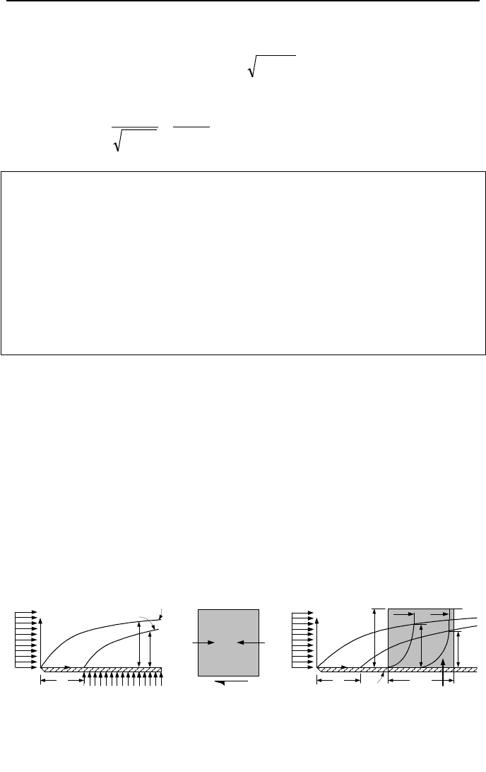
derive a relation for
δ’, we consider flow over a heated flat plate as shown in Fig-
ure IVb.2.1. This figure shows a case where heating of the plate starts at x = x
o
,
Figure IVb.2.1(a). For the derivation of a relation for
δ’, we may either reduce the
set of conservation equations of Chapter IIIa, for the control volume shown in
526 IVb. Heat Transfer: Forced Convection
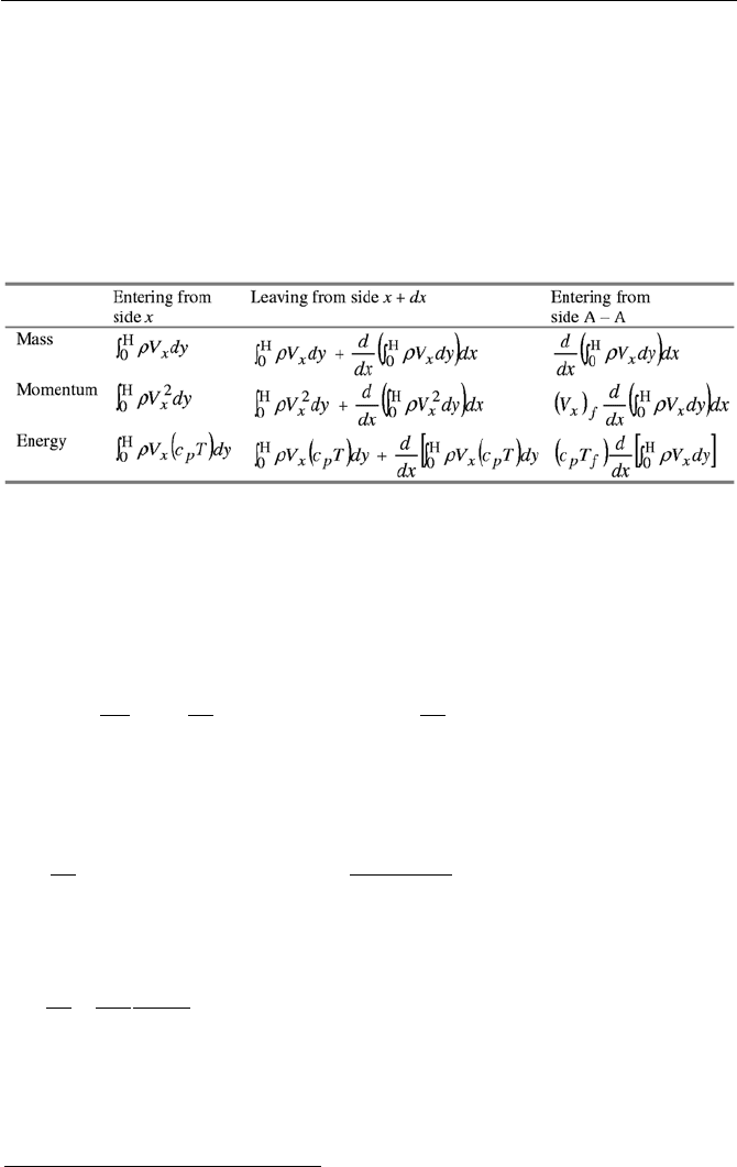
Figure IVb.2.1(c) or directly derive the conservation equations for this control
volume. Choosing the direct derivation by an integral approach
*
, we consider the
mass, momentum, and energy of the fluid entering and leaving this differential
control volume. These transfer processes enter from the vertical side located at x
and from the horizontal side (A-A) located in the free stream. Mass, momentum
and energy then leave the control volume through the vertical side located at x +
dx. These processes are summarized in Table IVb.2.1.
Table IVb.2.1. The transfer processes for the elemental control volume of Figure IVb.2.1
We first deal with the momentum equation for which at steady state, the resultant
of all forces is equal to the net momentum flux (i.e., the net momentum entering
minus the net momentum leaving the control volume, Equation IIIa.3.6). As
shown in Figure IVb.2.1(b), the forces applied on the control volume are the shear
at the solid surface and the pressure forces. The shear force at the free stream
(side A-A) is zero, thus:
=
¸
¹
·
¨
©
§
−− H
dx
dP
s
τ
³
()
dxdyV
dx
d
x
H
0
2
ρ
–
()
³
()
dxdyV
dx
d
V
x
f
x
H
0
ρ
IVb.2.5
We may simplify Equation IVb.2.5 by considering a case of constant pressure,
dP/dx = 0. The right side of Equation IVb.2.5 can also be simplified (see Prob-
lem 11) to obtain:
()
³
[]
y
yV
dyVVV
dx
d
x
sxxfx
∂
=∂
==−
)0(
)(
H
0
µτρ
IVb.2.6
If we substitute the velocity profile of Equation IVb.2.1 into Equation IVb.2.6 and
integrate, we conclude:
()
f
x
V
v
dx
d
13
140
į
į
= IVb.2.7
Equation IVb.2.7 can be integrated to obtain an approximate value for
δ. This
value differs by only 7.2% as compared with the exact value given by Equa-
tion IVb.2.4.
*
This method is originally developed by T. von Karman.

2. Analytical Solution 527
We now consider the energy equation for the differential control volume of
Figure IVb.2.1(c). The steady state form of Equation IIIa.3.9 relates the net en-
ergy addition to the control volume (by convection, conduction, and internal heat
generation as well as the viscous work) to net energy removal from the control
volume. Noting that the net viscous work is
µ
(∂V
x
/∂y)
2
dxdy (Example IIIa.3.12)
and considering only heat convection into and out of the control volume and heat
transfer from the solid surface, we find:
()
³
[]
s
x
p
xf
y
T
dy
dy
dV
c
dyVTT
dx
d
»
¼
º
«
¬
ª
∂
∂
=
»
»
¼
º
«
«
¬
ª
µ
µ
¶
´
¸
¸
¹
·
¨
¨
©
§
+−
α
ρ
µ
H
0
2
H
0
IVb.2.8
Note that in the derivation of Equation IVb.2.8, we made several assumptions in-
cluding steady state flow, fluid with constant properties, and the free stream with
constant velocity and temperature.
The rate of heat transfer from the surface, the right side of Equation Vb.2.8, can
be determined by substituting for the profiles of velocity and temperature from
Equations IVb.2.1 and IVb.2.2. However, the viscous dissipation term introduces
non-linearity, which precludes the development of an exact solution in closed
form. Fortunately, the net viscous work in laminar flow is generally negligible
compared with the rate of heat transfer by the convection or the conduction
mechanism. The viscous work becomes significant for high kinetic energy flows
or very viscous fluids.
Ignoring the net viscous work term, Equation IVb.2.8 simplifies to (see Prob-
lem 12):
()
αζ
ζ
ζ
10
į
įį
2
322
=
»
¼
º
«
¬
ª
+
dx
d
dx
d
V
f
x
where ȗ = δ’/δ. Introducing Equation IVb.2.7 and rearranging, we find the follow-
ing differential equation:
0
14
13
3
4
=−+
vdx
d
x
α
ξ
ξ
where ȗ = ȗ
3
. The boundary conditions for this differential equation is ȗ = 0 (since
δ’ = 0) at x = x
o
. Thus
3/1
4/3
3/1
1Pr
026.1
1
'
į
»
»
¼
º
«
«
¬
ª
¸
¹
·
¨
©
§
−==
−
x
x
į
o
ζ
IVb.2.9
If the plate is heated at the leading edge then
1/3
į '/ į ( Pr /1.026)
ζ
−
== .

528 IVb. Heat Transfer: Forced Convection
Determination of Heat Transfer Coefficient for Laminar Flow
over Flat Plate
Since h is defined as heat flux at the surface divided by
∆T, Equation IVb.1.1
gives:
fs
s
TT
yTk
h
−
∂∂−
=
)/(
We now need to find (∂T/∂y)
s
, which is obtained from Equation IVb.2.2. Substi-
tuting, we find:
)Pr026.1(
į2
3
'į2
3
)/(
3/1
kk
TT
yTk
h
fs
s
==
−
∂∂−
=
where we substituted for the thermal boundary layer thickness, δ’ in terms of the
hydrodynamic boundary layer thickness,
δ. We can further simplify this equation
by substituting for
δ from Equation IVb.2.4:
1/3 1/2 1/3 1/2 1/3
(/)
33
(1.026 Pr ) Re (1.026 Pr ) 0.3 Re (Pr )
2 į 25
s
sf
kT y
kk k
h
TT x x
−∂ ∂
== = =
−
Using the definition of the Nusselt number, Nu = hx/k, we find;
3/12/1
x
PrRe3.0Nu
x
= 0.6 < Pr < 50 IVb.2.10
Equation IVb.2.10 was derived analytically for the range of Pr number shown
above. However, we would have to resort to empirical correlations to be able to
include all fluids ranging from liquid metal (Pr in the order of 0.01) to motor oil
(Pr in the order of 50,000). One such correlation is that suggested by Churchill
and Ozoe:
3/12/1
PrReNu
xx
C= Re
x
Pr > 100 IVb.2.11
In Equation IVb.2.11, C is used to represent
[]
4/1
3/2
Pr)/(1/ baC += where coef-
ficients a and b for constant temperature are given as 0.3387 and 0.0468 and for
constant heat flux as 0.4637 and 0.0207. Thus, the Churchill and Ozoe correlation
for constant temperature is:
3/12/1
4/1
3/2
PrRe
Pr
0468.0
1
3387.0
Nu
xx
»
»
¼
º
«
«
¬
ª
¸
¹
·
¨
©
§
+
=
(T
s
= constant ) IVb.2.11-1
and for constant heat flux is:

2. Analytical Solution 529
3/12/1
4/1
3/2
PrRe
Pr
0207.0
1
4637.0
Nu
xx
»
»
¼
º
«
«
¬
ª
¸
¹
·
¨
©
§
+
=
(
constant=
′′
s
q
) IVb.2.11-2
The fluid properties in these correlations are developed at the film temperature.
Equations IVb.2.10 and IVb.2.11 demonstrate the dependency of the Nu num-
ber on Re and Pr numbers for laminar flow over a flat plate. These equations also
show that we should expect similar functional relationship for the Nu number even
if flow is not laminar. Thus for all practical purposes, we should expect:
32
PrReNu
1
c
c
c= IVb.2.11
where constants c
1
, c
2
, and c
3
depend on a specific case. Such functional relation-
ship between Nu, Re, and Pr numbers is indeed confirmed in many experiments
for forced convection heat transfer as discussed later in this chapter.
Determination of Average Heat Transfer Coefficient for Laminar Flow
over Flat Plate
To find the average heat transfer coefficient for laminar flow over a flat plate, we
note that in Equations IVb.2.11, the Nu number is a function of Re
1/2
. We may
then express the Nusselt number as Nu = C
1
Re
1/2
where C
1
represents all other
terms. Substituting for Re = V
f
x/v and for Nu = hx/k, we may write the heat trans-
fer coefficient as:
h
x
= (k/x)C
1
(V
f
x/v)
1/2
= B
1
x
–1/2
IVb.2.12
where B
1
= C
1
k(V
f
/v)
1/2
. If we now substitute for h
x
from Equation IVb.2.12 into
Equation IVb.1.2 and integrate over the entire length of the flat plate, we find the
average heat transfer coefficient as:
³
³
³
L
L
LL
x
hLBLLBLdxxBdxdxhh
0
2/1
1
2/1
1
2/1
1
00
22/2// =====
−−
Substituting for the heat transfer coefficient from h =Nu(k/x), we find
L
Nu2Nu = .
Example IVb.2.3. Water at high pressure and temperature flows over a heated
plat at 0.25 m/s. Temperature of water is 250 C and the plate temperature is main-
tained at 260 C. The length of the heated plate is 5 cm. Find the average heat flux
over the plate.
Solution: We find water properties at the film temperature T
film
= (250 + 260)/2 =
255 C
At T
film
= 255 C, v = 0.132E-6 m
2
/s, k = 0.6106 W/m·K, and Pr = 0.8458
Re
L
= VL/v = 0.25 × 0.05/0.132E-6 = 94,697. Flow is laminar so we use Equa-
tion IVb.2.11-1:

530 IVb. Heat Transfer: Forced Convection
C = 0.3387/[1 + (0.0468/0.8458)
0.666
]
0.25
= 0.327
Nu
L
= 0.312(94,697)
0.5
(0.8458)
0.333
= 95.28
h
L
= Nu
L
k/L = 95.28 × 0.6106/0.05 = 1163.6 W/m
2
·K
h = 2h
L
= 2 × 1163.6 = 2327 W/m
2
·K
=
′′
q
2327(260 – 250) = 23.27 kW/m
2
.
We now solve a similar example but for the flow of air over a heated flat plate.
In this example, we also find the thickness of the hydrodynamic boundary layer as
well as the thermal boundary layer.
Example IVb.2.4. A heated plate has a length of 0.5 m and width of 0.65 m. The
plate temperature is held constant at 119 C. Air at 15 m/s and 35 C flows over the
plate. Find a) the average heat transfer coefficient over the plate, b) total heat
transferred from the plate to the colder air and c) δ, and δ’ at the trailing edge.
Solution: We find air properties at the film temperature
T
film
= (35 + 115)/2 = 77 C
At T
film
= 75 C, v = 2.06E-5 m
2
/s, k = 0.0297 W/m·K, and Pr = 0.706
Re
L
= VL/v = 15 × 0.5/2.06E-5 = 364,077.
Flow is laminar so we use Equation IVb.2.11-1:
C = 0.3387/[1 + (0.0468/0.8458)
0.666
]
0.25
= 0.327
Nu
L
= 0.327(364,077)
0.5
(0.8458)
0.333
= 186
a) h
L
= Nu
L
k/L = 186 × 0.0297/0.5 = 11.08 W/m
2
·K
h = 2h
L
= 2 × 11.08 = 22.16 W/m
2
·K
b) =Q
22.16(0.5 × 0.65)(119 – 35) = 0.605 kW
c) 14.4077,364/5.05Re/5į
5.01/2
LL
=×=×= L mm
)Pr026.1/(į'į
3/1
= = 4.14/(1.026 × 0.706
0.3333
) = 4.53 mm.
So far we mostly dealt with the isothermal flow of fluids in the laminar flow
regime over a flat plate. For constant heat flux boundary condition see Problems
28 and 29. Next, we examine the internal laminar flow of fluids.
2.2. Internal Laminar Flow of Viscous Fluids
Velocity profile for fully developed, laminar flow in a pipe is a parabolic function
given by Equation IVb.2.1. Temperature profile for the same conditions can be
obtained from the two-dimensional steady state form of the conservation equation
of energy in the cylindrical coordinate system. Equation IIIa.3.23 assuming
steady state, no radiation heat transfer, no internal heat generation, no body force,
no viscous dissipation, and incompressible flow can be written as:

2. Analytical Solution 531
)( TkuV
o
∇⋅∇=∇⋅
K
K
K
K
ρ
Expanding this equation in two-dimensional cylindrical coordinates, while assum-
ing constant thermal conductivity, yields:
(
)
(
)
»
¼
º
«
¬
ª
¸
¹
·
¨
©
§
∂
∂
∂
∂
+
¸
¹
·
¨
©
§
∂
∂
∂
∂
=
»
¼
º
«
¬
ª
∂
∂
+
∂
∂
⋅+
x
T
xr
T
r
rr
ku
x
Tc
u
r
Tc
uVuV
x
p
r
p
xxrr
1
)(
GGGG
ρ
IVb.2.13
where
x
u
K
and
r
u
K
are the unit vectors. Since
x
u
K
is perpendicular to the conduit
flow area and hence to
r
u
K
, we find that 0=⋅=⋅
rxxr
uuuu
G
K
G
G
. If we also assume
that the fluid properties are weak functions of temperature, Equation IVb.2.13 re-
duces to:
¸
¹
·
¨
©
§
∂
∂
∂
∂
=
¸
¹
·
¨
©
§
∂
∂
+
∂
∂
r
T
r
rrx
T
V
r
T
V
xr
11
α
IVb.2.14
Equation IVb.2.14 is the same as Equation IIIa.3.23-1 but written in polar coordi-
nates. In Equation IVb.2.14 we have used the constant heat flux assumption,
0/ =
′′
dxqd
s
. This implies that the last term in the right side of Equation IVb.2.13
is equal to zero (i.e.,
∂(∂T/∂x)/∂x = 0). Since in the fully developed region, V
r
= 0
(and so is
∂V
x
/∂x = 0), Equation IVb.2.14 further simplifies to:
x
T
r
T
r
rrV
x
∂
∂
=
¸
¹
·
¨
©
§
∂
∂
∂
∂
α
11
IVb.2.15
To solve Equation IVb.2.15, we substitute the velocity profile for V
x
from Equa-
tion IVb.2.1 to obtain:
()
r
R
r
V
x
T
r
T
r
r
x
¸
¸
¹
·
¨
¨
©
§
−
∂
∂
=
¸
¹
·
¨
©
§
∂
∂
∂
∂
2
2
max
1
1
α
where R is the pipe radius. This equation can be easily integrated to find:
()
1
2
42
max
4
2
1
c
R
rr
V
x
T
r
T
r
x
+
¸
¸
¹
·
¨
¨
©
§
−
∂
∂
=
∂
∂
α
and the temperature distribution is finally obtained by another integration so that;
()
21
2
42
max
ln
16
4
1
crc
R
rr
V
x
T
T
x
++
¸
¸
¹
·
¨
¨
©
§
−
∂
∂
=
α