Massoud M. Engineering Thermofluids: Thermodynamics, Fluid Mechanics, and Heat Transfer
Подождите немного. Документ загружается.


332 IIIb. Fluid Mechanics: Incompressible Viscous Flow
In the analysis we often choose to simplify a piping network by substituting one
pipe to represent a series of pipes connected together. Thus, it is important to de-
termine the characteristics of the equivalent pipe.
Equivalent Pipe for Serial-Path and Parallel-Path Systems
To simplify the thermal-hydraulic analysis of a multi piping system connected in
series or in parallel, having different L, D
h
,
ε
and K, we substitute such a system
with an equivalent flow path (E). This substitution should be performed such that
the equivalent flow path retains the characteristics of the original system. Hence
the conservation equations of mass, momentum, and energy as well as the volume
constraint for the original system must also satisfy the equivalent flow path. The
volume constraint can be expressed in terms of equal transit time. As for the con-
servation equation of momentum, Equation IIIa.3.42 yields:
0)(hh)(
1V1
1212
=−+−+−+ ZZPP
gdt
d
A
L
g
pf
ρ
IIIa.3.42
We now apply the concept of equivalent flow path first to the serial and then to the
parallel systems.
Flow Paths Connected in Series
The continuity equation requires that
NiE
VVVV
1
"
"
===≡
. The energy
equation requires thermal properties to remain the same. The volume constraint
requires that
τ
E
= Σ
τ
i
where
τ
is the liquid transit time. Substituting for
τ
yields,
NNiiEE
V/VV/VV/VV/V
11
"
"
++≡
, which simplifies to:
¦¦
==
iiiE
ALVV IIIb.4.9
Applying Equation IIIa.3.42, the momentum equation to each pipe segment in
Figure IIIb.4.5(a), we obtain:
0)(hh)(
1V1
11
1
1
=−+−+−+
abpfab
ZZPP
gdt
d
A
L
g
ρ
#
IIIb.4.10
0)(hh)(
1V1
11
=−+−+−+
++ NNpNfNNN
N
N
ZZPP
gdt
d
A
L
g
ρ
adding up terms, we get:

4. Steady Incompressible Viscous Flow in Piping Systems 333
0)(hh)(
1V1
11
=−+−+−+
¸
¸
¹
·
¨
¨
©
§
++
¦¦¦
aNpifiaN
i
i
ZZPP
gdt
d
A
L
g
ρ
IIIb.4.11
We now apply Equation IIIa.3.42, the momentum equation to the equivalent flow
path:
0hh)(
1V1
1
=∆+−+−+
+ EpEfEaN
E
E
ZPP
gdt
d
A
L
g
ρ
IIIb.4.12
To have similar dynamic response, similar terms must be equal. Hence,
∆Z
E
≡
Z
N+1
– Z
1
,
¦
=
ipEp ,,
hh and
¦
=
i
i
E
E
A
L
A
L
IIIb.4.13
Additionally,
¦
=
fifE
hh , hence:
¦
=
2
V
)
K
(
2
V
)
K
(
2
2
*
2
2
*
E
ρρ
i
i
E
AA
IIIb.4.14
where in Equation IIIb.4.14, K
*
= fL/D + K. So far we have three equations;
Equations IIIb.4.9, IIIb.4.13, and IIIb.4.14. To find the five unknowns, V
E
, A
E
, L
E
,
D
E
, and K
E
we need two more equations. The fourth equation is obtained from V
E
= L
E
A
E
, as noted in Equation IIIb.4.9 and the fifth equation from the definition of
the hydraulic diameter:
wetted
Flow
h
S
A
D
V
4
P
4
wetted
== IIIb.4.15
Requiring equal wetted surfaces (S
wetted
) between the equivalent and the serial flow
paths and using Equations IIIb.4.9 and IIIb.4.14, we obtain the hydraulic diameter
of the equivalent pipe as:
,
,
(/)
ii
hE
ii hi
LA
D
LA D
=
Σ
Σ
IIIb.4.16
We now use the remaining three equations to find A
E
, L
E
, and K
E
. If we substitute
for A
E
in Equation IIIb.4.13 from A
E
= V
E
/L, to find
()
¦
=
iiEE
ALL /V/
2
and
then substitute for V
E
from Equation IIIb.4.9, we obtain:

334 IIIb. Fluid Mechanics: Incompressible Viscous Flow
()
5.0
»
»
¼
º
«
«
¬
ª
¦¦
¸
¸
¹
·
¨
¨
©
§
=
i
i
iiE
A
L
ALL
IIIb.4.17
having V
E
and L
E
, we can also express the flow area of the equivalent flow path,
A
E
as:
()
()
5.0
/
»
¼
º
«
¬
ª
¦
¦
=
ii
ii
E
AL
AL
A
IIIb.4.18
Finally, we find K
E
from Equation IIIb.4.14 as:
)(
K
K
2
*
2
E
E
E
i
i
EE
D
L
f
A
A −
»
»
¼
º
«
«
¬
ª
¦
=
IIIb.4.19
The results are summarized in Table IIIb.4.3.
Flow Paths Connected in Parallel
The volume constraint requires Equation IIIb.4.9 to be applicable here as well.
The momentum equation for each pipe segment in Figure III.8.1(b), is given by
the sets of Equation IIIb.4.10.
0h)(
1
V
1
11
1
1
1
=∆++−+ ZPP
gdt
d
A
L
g
fab
ρ
# IIIb.4.20
0h)(
1
V
1
=∆++−+
NfNab
N
N
N
ZPP
gdt
d
A
L
g
ρ
and for the equivalent flow path:
0h)(
1
V
1
=∆++−+
EfEab
E
E
E
ZPP
gdt
d
A
L
g
ρ
Pump terms are not shown as they develop equal heads. Since pressure terms are
equal, it requires that
dt
d
A
L
dt
d
A
L
dt
d
A
L
dt
d
A
L
N
N
N
E
E
E
V
VVV
2
2
21
1
1
"
===≡
IIIb.4.21
This results in finding each flow rate in terms of the equivalent pipe flow rate as:
E
i
i
E
E
i
d
L
A
A
L
d VV
¸
¸
¹
·
¨
¨
©
§
=
IIIb.4.22
4. Steady Incompressible Viscous Flow in Piping Systems 335
We now use, the mass balance requirement that:
NE
dddd VVVV
21
"
++=
IIIb.4.23
Substituting for each flow rate in terms of the equivalent pipe flow rate from
Equation IIIb.4.22 in Equation IIIb.4.23, we obtain:
()
¦
=
iiEE
LALA // IIIb.4.24
Canceling A
E
between V
E
= L
E
A
E
and Equation IIIb.4.24, we find an expression
for L
E
in terms of A
i
and L
i
:
()
()
5.0
/
»
¼
º
«
¬
ª
¦
¦
=
ii
ii
E
LA
AL
L
IIIb.4.25
Back substitution gives A
E
:
()( )
[]
5.0
/
¦¦
=
iiiiE
LAALA IIIb.4.26
To find the equivalent loss coefficient, from equal pressure drop requirement we
get:
2
2
2
1
2
1
1
1
1
1
2
2
2
V
K
2
V
K
2
V
K
N
N
N
N
N
i
E
E
E
E
E
E
gA
D
L
f
gA
D
L
f
gA
D
L
f
"
¸
¸
¹
·
¨
¨
©
§
+==
¸
¸
¹
·
¨
¨
©
§
+≡
¸
¸
¹
·
¨
¨
©
§
+
IIIb.4.27
We find each flow rate in terms of the flow rate in the equivalent path and substi-
tute it in the mass balance:
NE
VVVV
21
"
+++=
IIIb.4.28
we find:
() ( )
EENNEEEEE
AAAA V)/(K/KV)/(K/KV
2/1
**
1
2/1
*
1
*
"
++≡
where K
*
= K + (fL/D). Solving for K
E
, we get:
()
EEEiiE
E
DLfAA /K//K
2
*
−
»
¼
º
«
¬
ª
¸
¹
·
¨
©
§
=
¦
Finally, the hydraulic diameter for the equivalent pipe is obtained from Equa-
tion IIIb.4.16. The results are summarized in Table IIIb.4.3.

336 IIIb. Fluid Mechanics: Incompressible Viscous Flow
Table IIIb.4.3. Equivalent pipe characteristics
Example IIIb.4.12. Find the characteristics of an equivalent pipe to represent a
piping system connected in series. Individual pipe length, diameter, and loss coef-
ficients are given below. A flow rate of 100 GPM enters the piping system. Use
ρ
= 62.4 lbm/ft
3
and
µ
= 0.7E-3 lbm/ft⋅s. Pipe is smooth commercial steel.
Pipe No. L (ft) D (in) K (-)
1 100.00 3.50 5.00
2 180.00 3.00 4.00
3 50.00 2.50 6.00
4 90.00 2.00 1.00
Solution: We use Table IIIb.4.3 for pipes connected in series. Results are sum-
marized below:
Pipe LDAV K V
Re f ∆P
No. (ft) (in) (ft
2
) (ft/s) (-) GPM × 10
–6
(-) (psi)
1 100 3.5 0.067 3.32 5.00 100 0.087 0.0189 0.86
2 180 3.0 0.049 4.55 4.00 100 0.101 0.0184 2.39
3 50 2.5 0.034 6.55 6.00 100 0.121 0.0177 2.95
4 90 2.0 0.022 10.1 1.0 100 0.152 0.0169 7.12
Equivalent:
454.26 2.78 0.042 5.30 35.65 100 0.109 0.0181 13.3
Example IIIb.4.13. Find the characteristics of an equivalent pipe to represent a
piping system connected in parallel. Individual pipe length, diameter, and loss co-
efficients are given below. A flow rate of 19 lit/s enters the piping system. Use
ρ
= 998 kg/m
3
and
µ
= 1.1E-6 N·s/m
2
. Pipe is smooth commercial steel.
Pipe No. L (m) D (cm) K (-)
1 30.48 8.89 5.00
2 54.86 7.62 4.00
3 15.24 6.35 6.00
4 27.43 5.08 1.00
5. Steady Incompressible Viscous Flow Distribution in Piping Networks 337
X
1
X
2
X
3
X
4
X
5
X
6
X
7
X
10
X
11
X
13
X
14
X
12
X
15
X
9
X
8
Input Output
Output
Output
OutputOutputOutput
O
utput
M
X
2
PX
X
1
(a) (b)
Figure IIIb.5.1. (a) A piping network and (b) Example of a flow path details
Solution: We use Table IIIb.4.3 for pipes connected in parallel. Results are
summarized below:
Pipe LDA V K V
Re f ∆P
No. (m) (cm) (m
2
) (m/s) (-) lit/s × 10
–6
(-) (kPa)
1 30.48 8.89 6.207E-3 1.25 5.00 7.735 0.260 0.018 8.7
2 54.86 7.62 4.560E-3 1.00 4.00 4.613 0.303 0.018 8.7
3 15.24 6.35 3.167E-3 1.28 6.00 4.059 0.364 0.019 8.7
4 27.43 5.08 2.027E-3 1.22 1.00 2.516 0.455 0.019 8.7
Equivalent:
30.91 14.96 0.0175 1.08 11.5 18.92 0.292 0.016 8.7
5. Steady Incompressible Viscous Flow Distribution
in Piping Networks
In most engineering applications, fluid flows in multi-paths piping. Examples in-
clude water and gas distribution in municipalities, a nuclear plant emergency core
cooling system (ECCS), division of a PWR hot leg flow to steam generator tubes,
division of a BWR core flow rate between fuel bundles, and variety of piping sys-
tems in the balance of plant. In Section 4.4 we considered special cases of serial
and parallel piping systems. In this section, we consider more general case of pip-
ing networks, which may consists of a combination of serial and parallel piping
configurations.
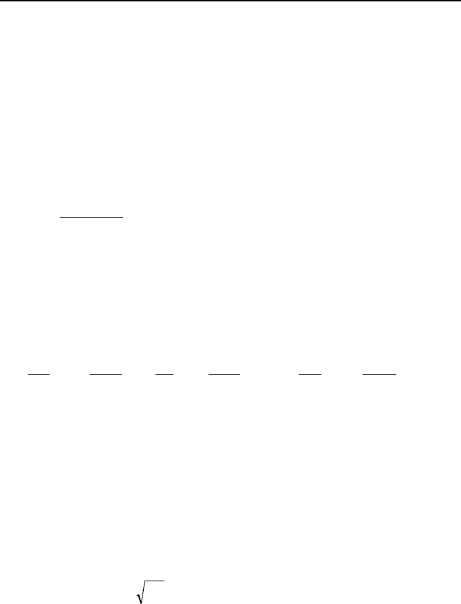
Figure IIIb.5.1(a) shows an example of a piping network consisted of loops and
nodes (X
1
through X
15
). A node is any point in the system at which either three or
more flows meet or network geometric dimensions change. A branch, link, or
flow path is referred to the conduits connecting two nodes. In general, a flow path
may also include pump, valves and fittings, as shown in Figure IIIb.5.1(b). Flow
paths that do not have circular flow area are modeled with the use of a hydraulic
diameter. Flow between various paths in a piping network is divided based on the
path resistance i.e. the least resistance path carries the most flow rate and vice

338 IIIb. Fluid Mechanics: Incompressible Viscous Flow
versa. A node may be connected to a boundary. There are two types of bounda-
ries namely, pressure boundary and flow boundary. Mathematically, these serve
as boundary conditions for the related differential equations. Flow boundaries are
of two types. A source-flow boundary, which supplies fluid to the network, and a
sink-flow boundary to which the nodal fluid flows. The sink fluid boundary is
also referred to as an output.
The goal is to find the steady-state nodal pressures and inter-nodal flow rates.
The boundary condition, generally include the output flow rates and either input
flow rate to or nodal pressure at the inlet of the network. In this example there are
15 unknown nodal pressures and 22 unknown branch flow rates. We have also 15
continuity equations and 22 inter-nodal momentum equations. There are 8 flow
boundary conditions (at nodes 1, 4, 9, 10, 11, 14, and 15). Of these, the flow to
node 1 is the supply flow and the rest are output flows.
To solve piping network problems, we seek simultaneous solution to a set of
continuity and momentum equations. The continuity equation is written for each
node and the momentum equation for each branch. Therefore, we obtain a set of
coupled non-linear differential equations, which are solved iteratively. In this
chapter we discuss three methods. The first two methods, known as Hardy Cross
and Carnahan method, are applicable to steady incompressible flow. The third
method, developed by Nahavandi, applies to both steady-state and transient in-
compressible flow. We discuss the first two methods here and leave the discus-
sion about the Nahavandi method to the transient flow analysis discussion in Sec-
tion 6.
The Hardy Cross Method
This method applies only to incompressible fluids, flowing under steady state and
isothermal conditions. In this method, the algebraic summation of all flow rates
associated with a node is set equal to zero. This results in as many equations as
the number of nodes. The reason for setting the summation of all flow rates asso-
ciated with a node equal to zero is that at steady-state, the conservation equation
for mass written for each node resembles the Kirchhoff’s law as applied to electric
circuits. According to the Kirchhoff’s law, the algebraic summation of nodal elec-
tric currents (flow rates) must be equal to zero:
0V
11
=
¦
=
¦
==
N
j
ji
N
j
ji
m
IIIb.5.1
where N is the number of branches stemming from a node, j is an index represent-
ing a branch to node i. In Figure IIIb.5.1, for example, N is equal to 15.
To find the flow distribution in the piping networks by the Hardy Cross
method, an initial best estimate is used to allocate flow rates to each loop compris-
ing the piping network. We then set the algebraic summation of the flow rates in
each loop equal to zero. Then a correction to the flow rate in each loop is applied
to bring the net flow rate into closer balance. Consider the piping network of Fig-

5. Steady Incompressible Viscous Flow Distribution in Piping Networks 339
ure IIIb.5.1. Suppose the initial guess in a branch is
0
V
. The correction to this
initial guess is
V
∆ such that the correct flow rate is now:
VVV
0
∆+=
IIIb.5.2
We use the estimated flow rate of each loop in the momentum equation for that
loop. We know that in a closed loop, we can write:
()
0=
¦
∆
j
j
P IIIb.5.3
Using Equation IIIb.3.6 for turbulent flow in a smooth pipe, pressure drop be-
comes a function of
8.1
V
. In general, pressure drop can be expressed as
V
n
Pc∆=
where n is some power depending on friction factor relation and c is
the proportionality constant as given in Equation IIIb.3.7. For example, if we treat
f as a constant then n = 2 and c = (fL/D)
ρ
/(2A
2
). Substituting for V
from Equa-
tion IIIb.5.2 and expanding terms according to the Taylor series, we obtain:
()
()
"
+∆+=∆+==∆
−
VVVVVV
1
000
nn
n
n
ncccP IIIb.5.4
If
V
∆ is small compared with
0
V
, we may ignore higher order terms not shown
in the right side of Equation IIIb.5.4 and apply this equation to a chosen loop in
the piping network, Equation IIIb.5.3, to get:
0VVVVVV
1
0
1
00
1
=
¦
∆+
¦
=
¦
=
¦
∆
−−− nnn
cnccP
IIIb.5.5
where first,
V
∆ is taken outside the summation since it is the same for the entire
loop and second, an absolute value sign is used to account for the flow direction.
We may choose an arbitrary direction for the flow but once chosen, use it consis-
tently. For example, we may choose all the clockwise flows as positive and all
counterclockwise flows as negative. From Equation IIIb.5.5 we find:
¦
¦
−=∆
−
−
1
0
1
00
V
VV
V
n
n
cn
c
IIIb.5.6
The solution procedure is as follows. We first use best engineering judgment to
allocate initial flow distribution to each loop. Next, we choose the flow directions
in each branch so that Equation IIIb.5.1 is satisfied at each node. We then assign
positive value to each branch flow rate in a loop that flows counterclockwise, for
example. Finally, we find the numerator and the denominator of Equation IIIb.5.6
to calculate the correction factor. Subsequently, we update flow rates using the
correction factor to calculate a new correction factor. We continue this process
until the calculated correction factor becomes exceedingly small.
340 IIIb. Fluid Mechanics: Incompressible Viscous Flow
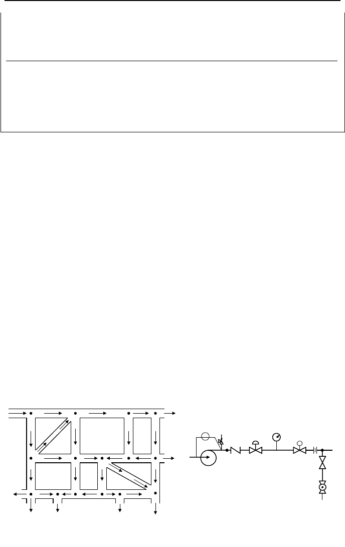
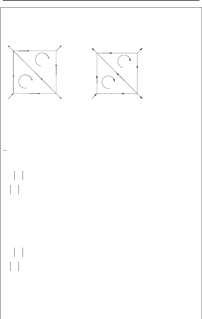
Example IIIb.5.1. Find flow distribution in the left side network, for n = 2. Units
of the c factors are such that the flow rates are in GPM (for example, for pipe with
c =2, 15V
2
=
=c
GPM, etc.).
c = 12
c = 10
c = 4
c =2
c
=
6
3
5
15
30
35
70
∆Q
1
∆Q
2
1
0
0
5
0
2
0
3
0
c = 12
c = 10
c = 4
c =2
c
=
6
1
.
5
1
4
29.241
52.272
20.759
47.728
∆Q
1
∆Q
2
1
0
0
5
0
2
0
3
0
Solution: We assume the clockwise direction as positive and use an initial guess
for the flow in each loop to be corrected in the following steps. We first correct
the assumed flow distribution in the lower loop:
1
c 6 10 12
0
V
35 –30 70
1
00
VV
−n
c
7350 –9000 58800 Summation: 57150
1
0
V
−n
cn
420 600 1680 Summation: 2700 −=∆
1
V
21.17
Updated
0
V
13.83 –51.17 48.83
We now update the upper loop as follows:
c 2 4 6
0
V
15 –35 –13.83
1
00
VV
−n
c
450 –4900 –1147.6 Summation: –5597.6
1
0
V
−n
cn
60 280 165.96 Summation: =∆
2
V
11.06
Updated
0
V
26.06 –23.94 –2.77
--------------------------------------------
In the second trial, we revise values in the lower loop, using the updated flow rate
for the common flow path:

5. Steady Incompressible Viscous Flow Distribution in Piping Networks 341
2
c 6 10 12
0
V
2.77 –51.17 48.83
1
00
VV
−n
c
46.04 –26183.69 28612.43 Summation: 2474.77
1
0
V
−n
cn
33.24 1023.4 1171.92 Summation: 2228.56 −=∆
1
V
1.11
Updated
0
V
1.66 –52.28 47.72
We now revise values in the upper loop flows, using the updated flow rate for the
common flow path:
c 2 4 6
0
V
26.06 –23.94 –1.66
1
00
VV
−n
c
1358.25 –2292.49 –16.53 Summation: –950.77
1
0
V
−n
cn
104.24 191.52 19.92 Summation: 315.68 =∆
2
V
3.01
Updated
0
V
29.07 –20.93 1.353
--------------------------------------------
We follow the same procedure in the third trial:
3
c 6 10 12
0
V
–1.353 –52.28 47.72
1
00
VV
−n
c
–10.98 –27,332 27,326 Summation: –16.6
1
0
V
−n
cn
16.23 1045.6 1145.28 Summation: 2228.56 −=∆
1
V
0.007
Updated
0
V
–1.345 –52.27 47.727
Revising the upper loop flows, using the updated flow rate for the common flow
path, in the third trial:
c 2 4 6
0
V
29.07 –20.93 1.345
1
00
VV
−n
c
1690.13 –1752.26 10.85 Summation: –51.27
1
0
V
−n
cn
116.28 167.44 –33.24 Summation: 250.48
=∆
2
V
0.168