Massoud M. Engineering Thermofluids: Thermodynamics, Fluid Mechanics, and Heat Transfer

Подождите немного. Документ загружается.

3. Set of Linear Equations 973

sponding rows – in other words, the coefficient matrix is diagonally dominant –

the convergence is guaranteed.

To demonstrate the Gauss – Seidel method, we try to solve the above set of lin-

ear equations. For this purpose, we obtain x

from the first, x

from the second,

and x

from the third equation – assuming nonzero coefficients – as follows:

3323213133

2232312122

1131321211

/)]([

axaxacx

+−=

VIId.3.4

To calculate x

from Equation VIId.3.4, for example, we need to have the val-

ues for x

and x

. Since we do not have these values before hand, we resort to

guessing based on the knowledge we have about the system of equations. Using

the initial guesses, we obtain updated values from Equation VIId.3.4. We con-

tinue this process and at each trial we compare the updated values with the previ-

ous values. If the difference is less than a specified convergence criterion then we

conclude that the iteration has converged. Using superscript k as an index of itera-

tion, the values of each parameter at iteration number k + 1 become:

)1(

313

)1(

)(

)1(

212

)1(

)(

121

)1(

/)]([

axaxacx

kkk

+++

+−=

Note that as soon as a new value for a variable is calculated, it is used to obtain the

new values for the rest of parameters. Let’s try this iterative method for the fol-

lowing set of linear equations:



=+−

−=−+

=++

113

542

zyx

For the first step we obtain:



−−=

−−−=

+−=

3/)](11[

4/)]2(5[

3/)](5[

yxz

zxy

zyx

To begin iteration, we may assume x = y = z = 0. From the first equation, new x

becomes x

(1)

= 1.666. From the second equation, new y becomes y

(1)

= [–5 –

(3.333 + 0)]/4 = –2.0833. From the third equation, new value for z becomes z

(1)

[11 – (1.666 + 2.0833)]/3 = 2.4168. We will use the updated values in the next

step of the iteration process as is summarized below. Note that k is the iteration

index:

974 VIId. Engineering Mathematics: Linear Algebra

k = 1 k = 2 k = 3 k = 4 k = 5 k = 6 k = 7 k = 8

0 1.666 1.555 1.2499 1.1195 1.0712 1.0370 1.0178

0 –2.083 –1.4235 –1.2065 –1.0978 –1.0656 –1.031 –1.0147

0 2.4168 2.6738 2.8478 2.880 2.9544 2.977 2.9892

As seen from this table, the values are approaching 1, –1, and 3 for x, y, and z, re-

spectively. The criterion for terminating the iteration is that:

−

old

new

where

is a specified convergence criterion, such as

101

−

× . As a result, to

solve a set of linear equations given by Ax = c, we develop the following algo-

rithm for the Gauss – Seidel iteration:

",2,1

)(

)1()1(

=−−=

¦¦

−

Solution to a set of equations can be easily found by using the software included

on the accompanying CD-ROM.

3.3. The Characteristic Equation of a Matrix

Mathematical modeling of engineering problems that are oscillatory in nature –

such as mechanical vibration and alternating current – leads to linear algebraic

systems of the type:

nnnnnn

xxaxaxa

=+++

2211

22222121

11212111

VIIc.1.16

or in the matrix form:

()

0=− xIA

VIIc.1.17

where A is the square matrix of coefficients, x is the vector of unknowns, I is the

identity matrix, and

is a parameter. According to Cramer’s rule, the only way

of having a nontrivial solution for the above homogeneous system is for the de-

terminant of the system of equations to be zero.

3. Set of Linear Equations 975

()

λλ

−

=−=

nnnn

aaa

IAP

22221

11211

det)( = 0 VIIc.1.18

The equation resulting from expansion of the above determinant is known as the

characteristic polynomial of matrix A. The roots of the characteristic polynomial

(

),,,

21 n

λλλ

" ) are referred to as the characteristic values or eigenvalues. Vec-

tors corresponding to the eigenvalues are referred to as characteristic vecors or ei-

genvectors.

976 VIIe. Engineering Mathematics: Numerical Analysis

VIIe. Numerical Analysis

In Chapter VIIIb, we studied analytical solutions of differential equations in

closed form. Despite all the advantages associated with analytical solutions, we

frequently have to resort to numerical solutions. This is due to the inability of

analytical methods to deal with the involved complexities in dealing with many

engineering problems. The primary advantage of analytical solutions is to provide

exact answers in functional relationships. The latter makes analytical solutions

independent of any specific problem to be analyzed. Numerical solutions, on the

other hand, are problem dependent. For example, any change in a boundary con-

dition requires the entire problem to be recalculated. Another key difference is

that numerical solutions provide answers only in tabulated form. On the plus side,

numerical solutions can handle complicated problems and therefore can, remove

the limitations inherent in analytical methods when dealing with nonlinearities.

Numerical methods can be divided into two groups: deterministic and statistic.

The deterministic group consists of such techniques as finite difference and finite

element. The statistical group deals primarily with such topics as the Monte Carlo

method. Finite difference methods, for example, are used to solve ordinary and

partial differential equations. Ordinary differential equations are solved based on

either the Taylor’s series technique or based on the predictor-corrector technique.

The Taylor’s series technique includes the Runge-Kotta and the Euler methods

while the predictor-corrector technique includes Adams, Moulton, Milne, and Ad-

ams Bashford methods. Partial differential equations can be divided into three

categories: Elliptic, Hyperbolic, and Parabolic. These equations are solved nu-

merically by either the explicit, semi-implicit, or fully implicit method. In this

chapter we consider only the finite difference methods.

1. Definiton of Terms

Accuracy. The reason this term is associated with numerical methods is that,

unlike analytical solutions, numerical methods are always associated with certain

degree of approximation. Accuracy is a measure of the closeness of the result ob-

tained from a numerical solution to an exact answer obtained from an analytical

solution. Although, in most cases, we do not have analytical answer to compare

with, reduction of errors associated with numerical solutions leads to increased ac-

curacy.

Backward difference. This definition is useful in the topic of interpolation.

Consider a set of y values associated with a specified set of x values as y

= f(x

For simplicity, let’s assume that all x values are equally spaced. We now define

the first-order backward difference as

)()(

1−

−=∇

iii

xfxff .

Central difference. For the same set of values described above, the central

difference is defined as:

1. Definiton of Terms 977

)

()

()(

xfxf

∆

−−

∆

Forward difference. For the same set of y values defined for backward differ-

ence, we may define the first-order difference as

)()(

1 iii

xfxff −=∆

. Simi-

larly, a second-order difference is defined as:

)]()([)]()([)()()]()([)(

11211

iiiiiiiiii

xfxfxfxfxfxfxfxfff −−−=∆−∆=−∆=∆∆=∆

+++++

Which simplifies to:

)()(2)(

iiii

xfxfxff +−=∆

Using the same procedure, we can find the nth order difference as:

)(

)2)(1(

)(

)1(

)()()(

321 −+−+−++

−−

−

+−=∆

ninininii

nnn

xnfxfxf

Round-off error. Most floating point operations involve some loss of sig-

nificant digits due to the finite word length of the computer. This loss of digits is

known as the round-off error. Arithmetic operations performed in single preces-

sion carry 7 or 8 significant digits for each variable. To reduce the round off error,

we use double precession, which nearly doubles the number of significant digits

assigned to the variable. The round-off error is also a function of the degree of the

involved arithmetic as well as the step size. The cumulative round-off error in-

creases as the step size is reduced.

Truncation error. In numerical analysis, we usually represent functions by a

limited number of terms of their expansions in Taylor’s series. As more terms in

the expansions are used, the truncation error is reduced.

Mesh size. The step size or mesh size is the increment applied to dependent

variables and is shown as

,x∆

,y∆ tz ∆∆ ,

, etc. The mesh size affects the discreti-

zation error. The smaller the mesh sizes, the smaller the discretization error, the

lager the number of arithmetic operations, and consequently the running time.

Discretization error. The discretization error stems from using a finite value

for the step size, such as

x∆ to represent an infinitesimal value, such as dx. The

discretization error is a direct function of the step size. The smaller the steps size,

the smaller the discretization error. On the other hand, as was discussed earlier,

the smaller the steps size, the larger the round off error. Therefore, there is basi-

cally an optimum value for the step size to have the minimum error, as shown in

Figure VIIe.1.1.

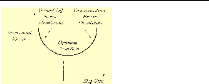
978 VIIe. Engineering Mathematics: Numerical Analysis

Figure VIIe.1.1. Depiction of dominance of numerical errors versus step or the increment

size

Local error. An error that appears in the calculation of a variable at a specific

step, of numerical integration for example, is known as the local error.

Propagated error. An error that appears in a step due to the accumulation of

errors of the successive steps is a propagated error. The propagated error is in ad-

dition to the local error corresponding to that step.

Numerical stability. If the propagated error is further accumulated as the nu-

merical process continues, a point may be reached where the error surpasses the

true value of the variable. This results in invalid values known as a numerically

unstable condition. A stable condition occurs where errors do not accumulate.

Nonlinear equation. An equation that contains multiples of a dependent vari-

able by itself or its derivatives, is a nonlinear equation. Such equations can be lin-

earized by the use of Taylor’s series.

Explicit numerical scheme: Approximation of a first order differential equa-

tion dy/dt = P(t)y + Q(t) in an explicit scheme is [y(t

n+1

) – y(t

)]∆t = P(t

)y(t

) +

Q(t

) where n is the discretization index.

The partial differential equations of parabolic type can be solved by forward

difference to explicitly calculate the dependent variable in terms of all the known

quantities. The size of increments in this scheme must remain below limit to

avoid numerical instability.

Implicit numerical scheme: Approximation of a first order differential equa-

tion dy/dt = P(t)y + Q(t) in fully implicit numerical scheme is [y(t

n+1

) – y(t

)]∆t =

P(t

n+1

+ Q(t

n+1

) where n is the discretization index. Approximation of the

above equation in semi-implicit scheme is [y(t

n+1

) – y(t

)]∆t = P(t

n+1

+ Q(t

Also the partial differential equations of a parabolic type can be solved by for-

ward difference to calculate the dependent variable in terms of all other dependent

variables, which are also unknowns. This requires successive simultaneous solu-

tion of sets of equations. The implicit scheme is unconditionally stable.

2. Numerical Solutions of Ordinary Differential Equations 979

2. Numerical Solutions of Ordinary Differential Equations

There are several methods for numerically solving the initial value problems of

ordinary differential equations among which we mention such method as Taylor’s

series, Euler, Adams, Adams-Bashforth, Adams-Moulton, Milne, and Runge-

Kutta. These methods can be basically divided into two groups. The first group

includes methods based on Taylor’s series. The second group are those based on

the “predictor-corrector” method.

2.1. Methods Based on Taylor – Series

Three such methods are discussed below including Taylor’s series, Euler, and

Runge-Kutta.

Taylor’s Series Method

To explain this method, we use a first order differential equation for which we can

readily find an exact answer by analytical means. We then use the Taylor’s Series

method to find an approximate solution for comparison with the exact solution to

determine the degree of approximation. Consider for example:

2 xy

=−

Subject to y(0) = 1/2. We may find the exact solution to this equation by using

Equation VIIb.2.4:

)

(

}]{[

++−=+=

³³

−−−

xxCeCdxexey

dxdx

where the method of “integration by part” was used twice to carryout the integral.

Applying the boundary condition, the exact solution becomes y = 0.75e

– 0.5(x

+ x + 0.5). Let’s now try the Taylor’s series method. In this method, the idea is to

find a relation between y and x. Such relation exists when we expand y in terms of

powers of x about the point x

by the Taylor’s series (Section VIIa.1). In this ex-

ample, since the boundary condition is given at x = 0, we may expand y about

x = 0 and use Maclaurin’s series to get:

′′′

∆

′′

∆

′

∆

+= )0(

)(

)0(

)(

)0(

)(

)0()(

321

yxy

Starting from x = x

, which in this case is x = 0, we can find y at any other interval

provided that we have y(0),

)0(y

′

, )0(),0( yy

′′′′′

, etc. We already have the first

value (i.e. y(0)) from the boundary condition. The second value,

)0(y

′

is found

from the differential equation itself as:

),(2

yxfxy

=+=

980 VIIe. Engineering Mathematics: Numerical Analysis

Hence 10)0(2)0( =+=

′

yy . The third and subsequent values are found from

successive derivation of the differential equation:

y 22)( +

′

′′

Since 1)0( =

′

y , then 2)0( =

′′

y . For the third value:

22)( +

′′

′′′

Since 2)0( =

′′

y , then 6222)0( =+×=

′′′

y . For the fourth derivative:

′′′

= 2)(

which gives 12)0( =

y . Similarly, for the fifth derivative;

ivivv

y 2)( ==

Therefore, y

(0) = 24. Let’s stop here and substitute the values we obtained in the

MacLaurin expansion of the function y to get:

)(

)()(

)(

errortruncationlocal

xxxxy +

∆

+∆+∆+∆+=

We can now set up the following table to summarize the comparison between ana-

lytical and numerical answers corresponding to various values of x. Note that the

increment of x values in Table VIIe.2.1 is 0.1.

These results indicate that we should have retained more terms in the Maclaurin

series to increase accuracy. The disadvantage of this method is that, for any prob-

lem, the derivatives must be carried out individually.

Table VIIe.2.1. Taylor – series method versus the analytical solution

x y

Taylor

Analytical

0.0 0.5 0.5

0.1 0.61052 0.611052

0.2 0.748864 0.748868

0.3 0.921536 0.921589

0.4 1.138848 1.139156

0.5 1.412500 1.413711

0.6 1.756352 1.760087

2. Numerical Solutions of Ordinary Differential Equations 981

The Euler Method

The Euler method is a simplified form of the Taylor’s series method where only

the first derivative is retained. This method is simple to use as no higher order de-

rivative needs to be carried out but, due to tendency to propagate local error, small

increments must be used. In the Euler method values of the function are obtained

at each increment or interval based on the value marching. To introduce the Euler

method, we can either use the Taylor –series with only the first two terms retained

or use Equation VIIb.2.1:

yxPxQ

)()( −=

VIIb.2.1

and approximate the derivative term:

),()()(

iiiii

yxfyxPxQ

=−=

∆

−

This is the explicit numerical scheme. The recursive formula is then given by:

xyxfyy

iiii

∆+=

),(

Let’s apply this method to the earlier example for which we already have solutions

from both the analytical and the Taylor’s series methods. In that example, we

have

2),( xyyxf += . The procedure is to start from the initial value we have,

which in this case is y(0) = 0.5, and calculate the successive values for y by using

an increment, of say,

.1.0=∆x This is summarized in Table VIIe.2.2.

Table VIIe.2.2. Euler method ( 1.0=∆x )

x y

f(x

, y

) y

n+1

0.1 0.5000 0.101 0.6010

0.2 0.6010 0.121 0.7252

0.3 0.7252 0.15404 0.87924

0.4 0.87924 0.191848 1.071088

0.5 1.071088 0.2392176 1.3103056

0.6 1.3103056 0.2980611 1.6083667

By comparing the result of the Euler method corresponding to 0.6 with the

Analytical solution we see that the error is nearly 9%. We then conclude that a

smaller interval should be used. Let’s try

01.0=∆x and summarize results in Ta-

ble VIIe.2.3. Note that the intermediate steps are not shown.

With the smaller increment, we improved the accuracy of the Euler method by

reducing the error to 1%. Data of Table VIIe.2.3 are produced by FORTRAN

Progarm VIIe.2.1, included on the accompanying CD-ROM.

982 VIIe. Engineering Mathematics: Numerical Analysis

Table VIIe.2.3. Euler method ( 01.0=∆x )

x y

f(x

, y

) y

n+1

0.0 0.5 1.0001 0.510001

0.1 0.510001 1.2056847 0.60989922

0.2 0.60989922 1.50221459 0.746129443

0.3 0.746129443 1.88558226 0.916646955

0.4 0.916646955 2.37480475 1.131150425

0.5 1.131150425 2.9930636724 1.4014624778

0.6 1.4014624778 3.7686172858 1.7419948229

The Runge-Kutta Methods

Another means of solving ordinary differential equations, also derived from the

methods based on the Taylor series expansion, is the Runge-Kutta methods.

These methods consist of four algorithms, which are similar in approach but differ

in the number of subintervals used in each interval. Like the Euler method, the

function is assumed to remain constant over a subinterval. The advantage of the

Runge-Kutta methods is the much higher order of truncation error obtained than in

the Euler method. The general form of the Runge-Kutta methods is:

),,(

xyxgxyy

iiii

∆∆+=

Where function ),,( xyxg

∆ depends on the specific Runge – Kutta method cho-

sen for the analysis. The simplest form for the function g is given by the three-

points Runge-Kutta method:

)

2/11 niiii

yxgxyy

′

∆

+∆+=

The third and fourth-order Runge-Kutta methods are equivalent to the Taylor’s se-

ries method carried as far as third and fourth derivatives, respectively. The four-

point of the third-order Runge-Kutta method is in the form of:

)4(

3211

kkk

∆

where k

, k

, and k

are given as

)2,(

)

(

),(

123

xkxkyxxfk

xfk

yxfk

∆−∆+∆+=

∆

The five-point of fourth-order Runge-Kutta method is in the form of:

)22(

43211

kkkk

+++

∆

where k

, k

, and k

are given as