Massoud M. Engineering Thermofluids: Thermodynamics, Fluid Mechanics, and Heat Transfer

Подождите немного. Документ загружается.

3. Numerical Solution of Partial Differential Equations 993

0))(1

()1

(

))(1

()1

()1(

,1,

,1,,,1

−×

∆

−

∆

−×

∆

−

∆

−

×∆

−

+−

jif

jiji

jif

jijijiji

VIIe.3.7

If the mesh sizes or increments are the same (

)yx ∆=∆ , we can simplify Equa-

tion VIIe.3.7 to get:

fjijijiji

TTT

∆

−=

∆

+−++

−+−

2)2(2)2(

,1,1,,1

VIIe.3.8

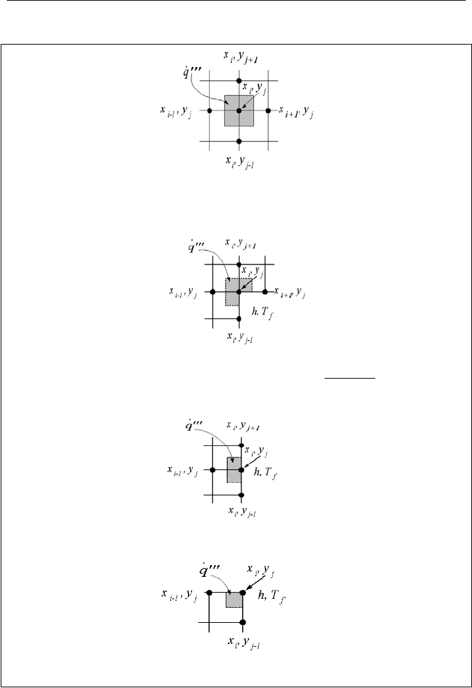
For the corner node with convection boundary and different heat transfer coeffi-

cients, Figure VIIe.3.5(c), we must consider heat conduction from half of the area

and heat convection from the rest of the area for nodes i – 1, j and i, j – 1:

1, , , 1 ,

, ,

(1)(1)()(1)(1)()0

22 22

i j ij ij ij

fij fij

TT TT

yy xx

k h TT k h TT

− −

−−

∆∆ ∆∆

×+×−+×+×−=

∆∆

ªºªº

«»«»

¬¼¬¼

Similarly, if the mesh sizes are the same ( )yx ∆=∆ , we can simplify this equation

to get:

fjijiji

∆

−=

∆

+−+

−−

2)1(2)(

,1,,1

VIIe.3.9

Two- Dimensional Temptionerature Distribution with Internal Heat Genera

We now derive similar algorithm for nodes considering internal heat generation in

these nodes. This includes an interior node, an interior corner node, a node at a

plane surface, and an external corner node.

Interior node (Figure VIIe.3.5):

)(

,1,1,,1,1

′′′

∆

+−+++

+−+−

TTTTT

jijijijiji



Internal corner node with convection boundary, Figure VIIe.3.6(a):

fjijijijiji

hhq

hhTTTT

∆

+−=

′′′

∆

++−+++

−++−

)(

)(3

])(6[)()(2

,211,,11,,1



Node at plane surface with convection boundary, Figure VIIe.3.6(b):

fjijijiji

TTT

∆

−=

′′′

∆

+−++

−+−

)(

)2(2)2(

,1,1,,1



994 VIIe. Engineering Mathematics: Numerical Analysis

For the corner node with convection boundary and different heat transfer coeffi-

cients, Figure VIIe.3.6(c):

fjijiji

hhq

hhTT

∆

+−=

′′′

∆

++−+

−−

)(

])(2[)(

,211,,1



These results are summarized in Table VIIe.3.1. A two-dimensional temperature

distribution in a solid with internal heat generation is solved in Section 10 of

Chapter IVa using the rectangular coordinates. We can use similar procedure to

solve problems in other orthogonal but not rectangular coordinates, such as cylin-

drical and spherical coordinates.

3.2. Parabolic Equations

Partial differential equations of the parabolic type are the most important equations in

the field of thermal science. The parabolic differential equations deal with physical

problems, which are time-dependent (also known as unsteady-state or transient) in

nature. As an example of a transient heat conduction problem, consider the same

problem shown in Figure VIIe.3.7 when one or several of the inputs changes with

time. This can either be due to a change in the ambient temperature (T

) with time,

change in the internal heat generation with time, or change in any of the boundary

temperatures with time. In the differential equations of the parabolic type, we have to

deal with space as well as time increments. In a three-dimensional problem, we have

four increments such as

,x∆

,y∆ ,z∆

and

t∆

. Since, in these types of problems, a

whole set of distribution for the unknown parameter, temperature for example,

changes from one time step to another, we then have to consider the concept of “val-

ues at the old time step” versus “values at the new time step”. This, in turn, brings up

the concept of explicit versus implicit methods. In the explicit method, the unknown

is defined only in terms of the known values, which are determined in the old or pre-

vious time step. In the implicit method on the other hand, all the values that are used

to determine the unknown are themselves expressed in the new time step. There is

also the semi-implicit method where, as the name implies, only some of the values

that determine the unknown are expressed in terms of the new time step.

An example of a one-dimensional parabolic differential equation includes time

dependent temperature distribution in a slender solid bar. In a slender bar, it is rea-

sonable to assume that each cross section can be represented with one temperature.

If the two ends are maintained at different but fixed temperatures, then temperature

varies only along the length of the bar. Now, suppose that temperature at one or

both ends begin to change with time. Temperature distribution along the length of

the bar will respond to this change and produce a time dependent profile for each

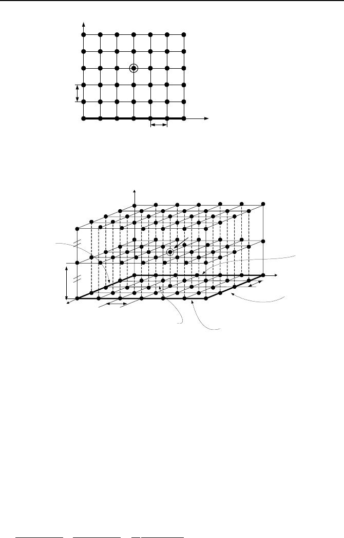
cross section along the length of the bar. Shown in Figure VIIe.3.8 is a schematic

representation of the space and time nodalization for determination of temperature

distribution in the solid bar. Functions f

(t) and f

(t) represent variation in tempera-

tures at both ends of the solid bar while f

(x) shows the initial temperature distribu-

tion in the bar before the end temperatures begin to change with time.

3. Numerical Solution of Partial Differential Equations 995

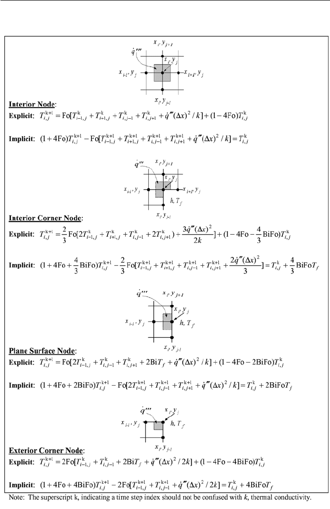
Table VIIe.3.1. Finite difference equations for two-dimensional transient heat conduction

Interior Node:

0]/)[(4

1,1,,1,1

=∆

′′′

+−+++

+−+−

kxqTTTTT

jijijiji



Interior Corner Node:

fji

jijijiji

Tkxh

TkxhTTTT )/(2)

)(3

()/)(3(2)()(2

1,,11,,1

∆−=

∆

′′′

+∆+−++++

−++−



Plane Surface Node:

fji

jijiji

TkxhkxqTkxhTTT )/(2]/)[()]/(2[2)2(

1,1,,1

∆−=∆

′′′

+∆++++

+−−



Exterior Corner Node:

fji

jiji

TkxhkxqTkxhTT )/(2]2/)[()]/(1[2)(

1,,1

∆−=∆

′′′

+∆+−+

−−



996 VIIe. Engineering Mathematics: Numerical Analysis

∆x

∆t

T(0, j) = f

)

T(m, j) = f

)

i, j

Boundary Condition:

Initial Condition: T(i, 0) = f

)

Figure VIIe.3.7. One-dimensional transient temperature distribution in a solid bar

∆ y

∆ t

∆ x

T(i, j, k)

Boundary Condition:

T(i, 0, 0) = f

)

Boundary Condition:

T(0, j, 0)=f

)

Initial Condition:

T(i, j, 0) = f

, y

)

Boundary Condition:

T(i, n, 0)=f

)

Boundary Condition:

T(m, j, 0)=f

)

Figure VIIe.3.8. Two-dimensional transient temperature distribution in a plate

Similar discussion is applicable to a two-dimensional parabolic partial differen-

tial equation. For example, consider temperature distribution in the plate of Fig-

ure VIIe.3.8. Initially, temperature at the four boundaries are specified and the

steady-state temperature distribution in the plate is given as f

(x, y). Then one or

all of the four boundary temperatures are allowed to change with time. Nodal

temperatures within the plate then become functions of x, y, and t.

Explicit and Implicit Numerical Schemes

The concepts of explicit and implicit numerical schemes appear when we try to

discretize the differential terms. Let’s consider the heat conduction equation de-

scribing time dependent temperature distribution in the plate of Figure VIIe.3.8:

tyxT

∂

∂ ),,(1),,(),,(

VIIe.3.10

3. Numerical Solution of Partial Differential Equations 997

We now begin to discretize the differential terms in finite difference. The more

straightforward term to tackle is the time derivative term, which describes the rate

of change of nodal temperature. In other words, this term describes the difference

between nodal temperature in the new time step and the previous time step. Here,

for the sake of consistency, we use the same notation as used in Figure VIIe.3.8.

Subscripts i and j are used to represent nodal temperature in the x and y directions,

respectively. The range of subscript i is from 0 to m and the range of subscript j is

from 0 to n. Superscript k is used to represent nodal temperature at the previous

time step and k + 1 for nodal temperature at the new time step:

tyxT

∆

−

∂

),,(

VIIe.3.11

Having discretized the temporal term, we now proceed to discretize the spatial

terms. For this purpose, we may use the forward difference method where each

nodal temperature is described in terms of its adjacent nodes as done in Equa-

tion VIIe.3.10:

∂

),(),(

yxT

1,,1,

,1,,1

)(

TTT

jijijijijiji

∆

+−

∆

+−

+−+−

What is missing in this expression is the lack of reference to time, as this expres-

sion is applicable to the steady-state condition. If we express all the above tem-

peratures to correspond to the current time step:

∂

),,(),,(

tyxT

1,,1,

,1,,1

)(

TTT

∆

+−

∆

+−

+−+−

VIIe.3.12

and substitute Equations VIIe.3.12 and VIIe.3.11 into Equation VIIe.3.10, we can

find temperature of node i, j at the next time step (

T ) explicitly in terms of

nodal temperatures at the current time step:

1,,1,

,1,,1

)(

TTT

∆

+−

∆

+−

+−+−

∆

−

If we assume that

yx ∆=∆

and we also replace Fo)/(

=∆∆ xt

, the above ex-

pression simplifies to:

TTTTTT

,1,1,,1,1

)Fo41()(Fo −++++=

+−+−

VIIe.3.13

Equation VIIe.3.13 provides the algorithm that allows us to calculate the nodal

temperature of the new time step in terms of all the known temperatures of the

previous time step. To compare this explicit approach with the fully implicit ap-

proach, we use the same equations and the same substitutions but develop the spa-

998 VIIe. Engineering Mathematics: Numerical Analysis

tial finite difference in Equation VIIe.3.12 with temperatures that correspond to

the new time step to get:

)(

TTT

∆

+−

∆

+−

−

∆

−

If we assume that

yx ∆=∆

and we also replace Fo)/(

=∆∆ xt

, the above ex-

pression simplifies to:

TTTTTT

)(Fo)Fo41( =+++−−

−

VIIe.3.14

In Equation VIIe.3.14 the intended nodal temperature as well as all the neighbor-

ing temperatures are unknown. Equation VIIe.3.14 provides the algorithm to de-

velop a set of algebraic equations, which should be solved simultaneously to find

nodal temperatures corresponding to the new time step.

Stability of Explicit and Implicit Schemes

Comparing Equations VIIe.3.13 and VIIe.3.14, we see that the nodal temperature

for the new time step in the explicit scheme is readily calculated in terms of

known temperatures of the previous time step as opposed to the implicit scheme

where sets of algebraic equations must be solved in each time step. On the other

hand, the implicit scheme is unconditionally stable whereas in the explicit scheme

we must ensure the spatial and temporal increments are small enough to obtain

convergence and calculate meaningful physical quantities. As a result, to prevent

instability due to the numerically induced oscillations, it can be both physically

and mathematically shown that in Equation VIIe.3.13 we must have 1 – 4Fo

≥ 0.

Hence, the condition for stability in the explicit numerical scheme requires that Fo

≤ 1/4 or equivalently ∆t ≤∆x

. This implies that in solving two-dimensional

problems by the explicit scheme, once the spatial increment is chosen, the tempo-

ral increment must remain smaller than the square of the spatial increment divided

by 4

Derivation of Finite Difference Formulation for Nodal Temperature

Earlier we derived the finite difference formulation of the nodal temperatures from

the heat conduction equation VIIe.3.10. We may derive the same formulation in

both explicit and implicit schemes from the energy balance for each node. For ex-

ample, for an interior node, as shown in Figure VIIe.3.4, we write:

Total rate of heat transfer into the node + Rate of internal heat generation in the

node = Rate of change of nodal internal energy

We can substitute for each term, in either an explicit or implicit manner. For ex-

ample, if we develop terms implicitly we get:

3. Numerical Solution of Partial Differential Equations 999

cyxyxq

∆

−

×∆×∆=×∆×∆

′′′

∆

−

×∆+

∆

−

×∆+

∆

−

×∆+

∆

−

×∆

−

)1()1(

)1()1()1()1(



Note that, in this derivation we have assumed a constant rate of heat generation

and thermal properties that are independent of temperature. In general, thermal

properties are temperature dependent and the rate of internal heat generation may

change with time. In this case, we should also develop such terms in a discretize

manner based on the constitutive equations explaining each term, which is rather

straightforward in the explicit scheme. However, in the implicit scheme, devel-

opment of the related constitutive equations would lead to the appearance of

nonlinear terms, which should be linearized. Returning to the above equation, if

we assume

yx ∆=∆

and make use of the definition of thermal diffusivity, we ob-

tain Equation VIIe.3.14 with an additional term representing the internal heat gen-

eration. Using the derivation method described here, we can derive similar rela-

tions for interior corner, plane surface, and external corner nodes as shown in

Figure VIIe.3.5. The derivation is left as an exercise to the reader. The results are

summarized in Table VIIe.3.2.

Note that in Table VIIe.3.1, a constant internal heat generation is assumed. If

there is no internal heat generation, then the volumetric heat generation rate (i.e.

term

′′′



) should be set equal to zero. Also note that if a boundary is insulated

rather than being exposed to a convection boundary, the heat transfer coefficient

can be viewed as being zero. Hence, for insulated, adiabatic, or symmetric sur-

faces, the Bi in equations of Table VIIe.3.2 must be set equal to zero.

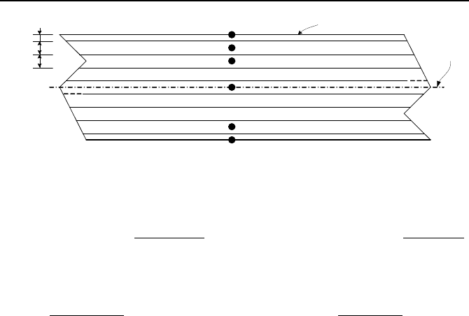
Slab Exposed to Convection Heat Transfer at the Boundary

As an example, let’s consider the implicit formulation for temperature distribution

in a slab of a specified initial temperature exposed to convection heat transfer at its

boundaries. The formulation may take into account hetrogenous internal heat

generation and material (i.e., both

′′′



and k are functions of location). As shown

in Fingure VIIe.3.9, the slab is divided into N regions. The thickness of the inte-

rior regions is

∆x and the thickness of the boundary regions is ∆x/2. Thus, the in-

terior nodes are located in the center of the interior regions. Due to the symmetry,

we may write the energy equations for only half of the slab and apply an adiabatic

boundary to the center of the slab. The energy equation for the ith interior node

becomes:

()

cxxq

∆

−

×∆×=∆×

′′′

∆

−

∆

−

k1k

1k1k



Next, we consider the energy equation for the boundary nodes, nodes 1 and m.

1000 VIIe. Engineering Mathematics: Numerical Analysis

∆x

∆x/2

N-1

h, T

Adiabatic

boundary

Figure VIIe.3.9. Schematic of a slab exposed to convection boundary

For node 1, exposed to heat transfer by convection, we write:

()

cxxq

kTTh

∆

−

×∆×=∆×

′′′

∆

−

+−

2/2/



and for node m, located on an adiabatic boundary, we write:

()

cxxq

∆

−

×∆×=∆×

′′′

∆

−

k1k

1k1k

2/2/



wkere k is thermal conductivity and k, as the superscript, is an index to advance

time. Writing the energy equation for all the interior nodes, we can summarize the

results in the following matrix equation:

+−

−+−

−++

Fo1Fo2000

FoFo21Fo

0Fo2Fo1Fo0

00Fo2Fo1Fo

000FoFoBi2Fo21

"""

"""""

−

FoBi2

Starting at time zero (the superscript k = 0), all the nodal temperatures are known.

Thus, we solve the above equation for nodal temperatures when time is advance

one time step. We continue the solution to until the end of the specified transient

time is reached. The accuracy of temperature distribution increases as the number

of nodes increases. This however, means that the array sizes to hold the matrix

elements increases as we must inverse larger coefficient matrices at each time

step.

3.3. Hyperbolic Equations

Partial differential equations of the hyperbolic type appear basically in problems

involving vibration and wave motion. As such, problems in waterhammer, neu-

tron diffusion, radiation transfer, and supersonic flow are examples of hyperbolic

3. Numerical Solution of Partial Differential Equations 1001

differential equations. The general form of the wave equation is given by Equa-

tion VIIb.1.31 and the one-dimensional equation in the Cartesian coordinate sys-

tem is given in Equation VIIb.1.31-1 and repeated here:

),(1),(

txy

∂

VIIe.3.15

where

Tgc = . If we now use an explicit numerical scheme, the finite dif-

ferential form of Equation VIIe.3.15 for node i at time k + 1 becomes:

)(

yyy

∆

+−

∆

+−

Solving for the displacement at the new time step:

yyyy

−

+−= VIIe.3.16

where in this derivation we have taken the value of the coefficient as unity (i.e.

1)/()(

222

=∆∆ xtc ). From here, the time step size becomes:

∆

=∆

It turns out that the time step calculated above is indeed the optimum time step

size with respect to stability and convergence. An interesting feature of Equa-

tion VIIe.3.16, which involves a second derivative with respect to time, is the ap-

pearance of the lateral movement prior to time zero (i.e. term y

–1

). Obviously, we

find y

from the boundary condition. But we need to have another condition to

find y

–1

. One way is to use the initial velocity (i.e. 0/)0,( =∂=∂ ttxy

). Using

the central-difference approximation, we find:

∆

−

Substituting into Equation VIIe.3.16 to eliminate y

–1

, we get displacement of the

first time step as:

)(

+−

iii

yyy

Having displacement at the first time step in terms of displacements at time zero,

we can proceed to find all other displacements at successive time steps from Equa-

tion VIIe.3.16.

1002 VIIe. Engineering Mathematics: Numerical Analysis

Table VIIe.3.2. Finite difference equations for two-dimensional transient heat conduction