Lee K.K. Lectures on Dynamical Systems, Structural Stability and Their Applications
Подождите немного. Документ загружается.

relating
to
local
geometric
properties
in
the
neighborhood
of
points,
lines,
surfaces
or
manifolds
in
general.
In
global
differential
geometry,
by
contrast,
one
is
interested
in
the
integrals
of
those
local
differential
relations
and
questions
arise
whether
those
integrals
exist
and
whether
they
are
unique.
For
lower
dimensional
spaces
(n
~
3)
there
is
a
well
balanced
relationship
between
local
and
global
results
in
differential
geometry
(e.g.,
Gauss-Bonnet
theorem).
However,
for
higher
dimensional
space,
it
is
much
more
difficult
to
generalize
the
local
results
to
global
ones.
In
Newtonian
or
Poincare-invariant
theories
the
space-time
is
considered
to
be
given
a
priori,
and
the
physical
dynamics
are
defined
on
this
background.
In
general
relativity,
the
topological
and
geometric
structure
of
space-time
is
to
be
established
as
part
of
the
dynamics.
Global
structures
place
restrictions
on
the
class
of
differentiable
manifolds
suitable
for
space-times.
Global
structures
are
presented
in
mathematical
form
but
their
imposition
is
usually
based
upon
physical
intuition
and
on
observations.
once
they
are
imposed,
however,
the
resultant
class
of
admissible
spaces
further
clarifies
the
significance
of
any
given
global
structure
and
could
even
lead
to
its
rejection.
Before
getting
into
formal
definitions
and
major
results,
let
us
describe
the
concepts
we
shall
encounter
in
an
intuitive
way.
We
have
defined
the
tangent
space
of
a
manifold
Mat
a
point
p £
M,
i.e.,
MP.
The
tangent
bundle
of
M,
denoted
by
TM,
is
defined
as
the
union
of
all
tangent
spaces
of
M,
i.e.,
TM
= U
~for
all
p £
M.
A
vector
bundle
of
a
manifold
M
is
a
family
of
vector
spaces
V
each
attached
to
a
point
of
M
such
that
locally
the
vector
bundle
is
homeomorphic
to
u x V
where
U
is
a
neighborhood
of
p £
M.
The
principal
bundle
of
M
with
structural
group
G
is
locally
homeomorphic
to
the
attachment
to
each
point
in
M a
different
copy
of
G,
i.e.,
the
bundle
is
locally
homeomorphic
to
U x G
where
U
is
a
neighborhood
of
p £
M.
we
84
say
a
bundle
is
trivial,
we
mean
that
instead
of
the
bundle
space
"is
locally
homeomorphic
to"
by
"is
homeomorphic
to".
In
the
following,
we
shall
discuss
fiber
bundles
on
a
smooth
manifold
with
smooth
mappings.
These
notions
are
very
useful
for
our
discussion
as
well
as
for
differential
geometry.
But
it
should
be
pointed
out
that
fiber
bundles
can
be
defined
on
topological
manifolds
only
with
all
maps
continuous
[Steenrod
1951].
For
example,
let
B,
X
and
F
are
topological
manifolds
and
let
a
continuous
map
~
: B
~
X
of
B
onto
X
called
the
projection
and
B
be
the
bundle
space
and
X
the
base
space.
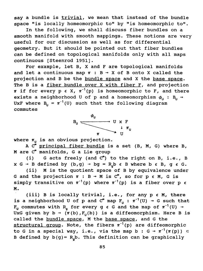
The
B
is
a
fiber
bundle
over
X
with
fiber
F,
and
projection
~
if
for
every
p E
X,
~-
1
(p)
is
homeomorphic
to
F,
and
there
exists
a
neighborhood
U
of
p
and
a
homeomorphism
¢u :
Bu
~
UxF
where
Bu
=
~-
1
(U)
such
that
the
following
diagram
commutes
¢u
where
~u
is
an
obvious
projection.
X F
.1.
~u
u
A
c-
principal
fiber
bundle
is
a
set
(B,
M,
G)
where
B,
M
are
c-
manifolds,
G a
Lie
group
(i)
G
acts
freely
(and
c-)
to
the
right
on
B,
i.e.,
B
X G
~
B
defined
by
(b,g)
~
bg
= R
9
b E B
where
b E
B,
g E
G.
(ii)
M
is
the
quotient
space
of
B
by
equivalence
under
G
and
the
projection
~
: B
~
M
is
c-,
so
for
p e
M,
G
is
simply
transitive
on
~-
1
(p)
where
~-
1
(p)
is
a
fiber
over
p e
M.
(iii)
B
is
locally
trivial,
i.e.,
for
any
p
eM,
there
is
a
neighborhood
U
of
p
and
c-
map
Fu
:
~-
1
(U)
~
G
such
that
Fu
commutes
with
R
9
for
every
g e G
and
the
map
of
~-
1
(U)
~
UxG
given
by
b
~
(~(b),Fu(b))
is
a
diffeomorphism.
Here
B
is
called
the
bundle
space,
M
the
base
space,
and
G
the
structural
group.
Note,
the
fibers
~-
1
(p)
are
diffeomorphic
toG
in
a
special
way,
i.e.,
via
the
map
b : G
~
~-
1
(~(p))
c
B
defined
by
b(g)=
R
9
b.
This
definition
can
be
graphically
85
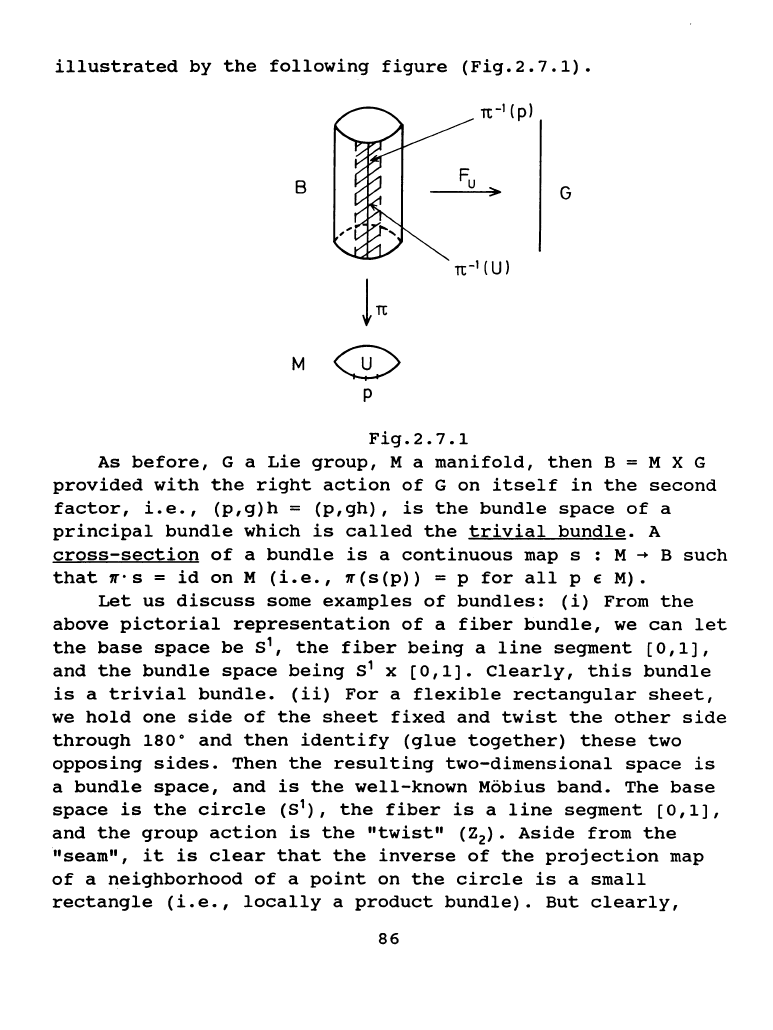
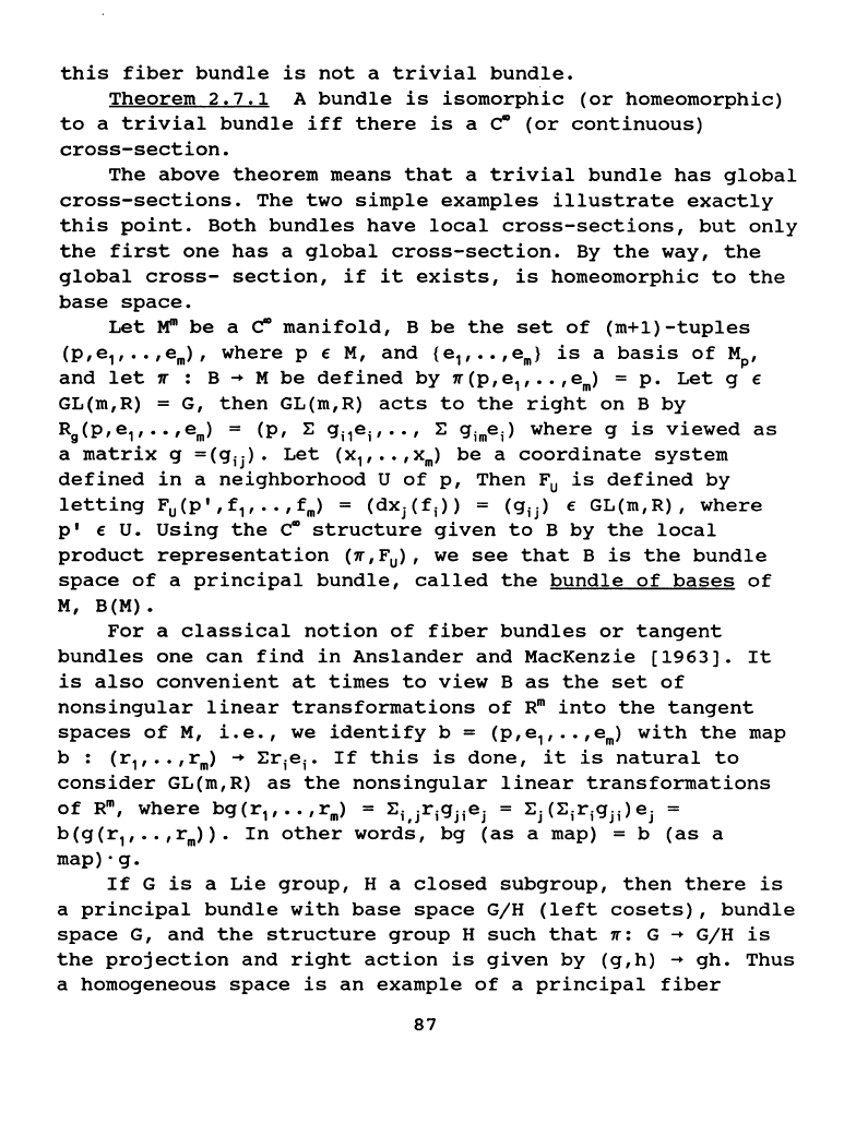
illustrated
by
the
following
figure
(Fig.2.7.1).
B
G
Fig.2.7.1
As
before,
G a
Lie
group,
M a
manifold,
then
B = M X G
provided
with
the
right
action
of
G
on
itself
in
the
second
factor,
i.e.,
(p,g)h
=
(p,gh),
is
the
bundle
space
of
a
principal
bundle
which
is
called
the
trivial
bundle.
A
cross-section
of
a
bundle
is
a
continuous
map s : M
~
B
such
that
r·s
=
id
on
M
(i.e.,
r(s(p))
= p
for
all
p
eM).
Let
us
discuss
some
examples
of
bundles:
(i)
From
the
above
pictorial
representation
of
a
fiber
bundle,
we
can
let
the
base
space
be
s
1
,
the
fiber
being
a
line
segment
[0,1],
and
the
bundle
space
being
s
1
x
[0,1].
Clearly,
this
bundle
is
a
trivial
bundle.
(ii)
For
a
flexible
rectangular
sheet,
we
hold
one
side
of
the
sheet
fixed
and
twist
the
other
side
through
1so•
and
then
identify
(glue
together)
these
two
opposing
sides.
Then
the
resulting
two-dimensional
space
is
a
bundle
space,
and
is
the
well-known
Mobius
band.
The
base
space
is
the
circle
(S
1
),
the
fiber
is
a
line
segment
[0,1],
and
the
group
action
is
the
"twist"
(Z
2
).
Aside
from
the
"seam",
it
is
clear
that
the
inverse
of
the
projection
map
of
a
neighborhood
of
a
point
on
the
circle
is
a
small
rectangle
(i.e.,
locally
a
product
bundle).
But
clearly,
86
this
fiber
bundle
is
not
a
trivial
bundle.
Theorem
2.7.1
A
bundle
is
isomorphic
(or
homeomorphic)
to
a
trivial
bundle
iff
there
is
a
c-
(or
continuous)
cross-section.
The
above
theorem
means
that
a
trivial
bundle
has
global
cross-sections.
The
two
simple
examples
illustrate
exactly
this
point.
Both
bundles
have
local
cross-sections,
but
only
the
first
one
has
a
global
cross-section.
By
the
way,
the
global
cross-
section,
if
it
exists,
is
homeomorphic
to
the
base
space.
Let~
be
a
c-
manifold,
B
be
the
set
of
(m+1)-tuples
(p,e
1
,
••
,em),
where
p E
M,
and
{e
1
,
••
,em}
is
a
basis
of
MP,
and
let~:
B
~
M
be
defined
by
~(p,e
1
,
••
,em)
=
p.
Let
g e
GL(m,R) =
G,
then
GL(m,R)
acts
to
the
right
on
B
by
R
9
(p,e
1
,
••
,em) =
(p,
~
g;
1
ei'
•.
,
~
gime;)
where
g
is
viewed
as
a
matrix
g
=(g;j).
Let
(x
1
,
••
,xm)
be
a
coordinate
system
defined
in
a
neighborhood
U
of
p,
Then
Fu
is
defined
by
letting
Fu(P',f
1
,
••
,fm) =
(dxi(f;))
=
(g;j)
E
GL(m,R),
where
p'
e U.
Using
the
c-
structure
given
to
B
by
the
local
product
representation
(~,Fu),
we
see
that
B
is
the
bundle
space
of
a
principal
bundle,
called
the
bundle
of
bases
of
M,
B(M).
For
a
classical
notion
of
fiber
bundles
or
tangent
bundles
one
can
find
in
Anslander
and
MacKenzie
[1963].
It
is
also
convenient
at
times
to
view
B
as
the
set
of
nonsingular
linear
transformations
of
Rm
into
the
tangent
spaces
of
M,
i.e.,
we
identify
b =
(p,e
1
,
••
,em)
with
the
map
b :
(r,
••
,
rm)
~
~r;e;.
If
this
is
done,
it
is
natural
to
consider
GL(m,R)
as
the
nonsingular
linear
transformations
of
Rm,
where
bg
(r
1
,
••
,
rm)
=
~i.irigiiei
=
~i
(~;r;gji)
ei
b(g(r
1
,
••
,rm)).
In
other
words,
bg
(as
a map) = b
(as
a
map)·g.
If
G
is
a
Lie
group,
H a
closed
subgroup,
then
there
is
a
principal
bundle
with
base
space
G/H
(left
cosets),
bundle
space
G,
and
the
structure
group
H
such
that
~=
G
~
G/H
is
the
projection
and
right
action
is
given
by
(g,h)
~
gh.
Thus
a
homogeneous
space
is
an
example
of
a
principal
fiber
87
bundle.
[Helgason
1962,
Steenrod
1951].
Let
(B,M,G)
be
a
principal
bundle
and
let
F
be
a
manifold
on
which
G
acts
to
the
left.
The
fiber
bundle
associated
to
CB.M.Gl
with
fiber
F
is
defined
as
follows:
Let
P
1
= B x
F,
andconsider
the
right
action
of
G
on
P
1
by
(b,f)g
=
(bg,g"
1
f)
where
b E
8,
f E
F,
g E G.
Let
P = P
1
/G,
the
quotient
space
under
equivalence
by
G,
then
P
is
the
bundle
space
of
the
associated
bundle.
The
projection
~
1
:
P
~
M
is
defined
by
~
1
((b,f)G)
=~(b).
For
p
eM,
we
take
a
neighborhood
U
of
p
as
in
(iii)
of
the
definition
of
a
principal
bundle,
with
Fu:
~-
1
(U)
~
G.
Likewise
we
have
Fu
1
:
~
1
(U)
~
F
by
Fu
1
((b,f)G)
=
Fu(b)f
so
that
(~
1
)"
1
(U)
is
homeomorphic
to
U x
F,
and
define
P
as
a
manifold
by
requiring
these
homeomorphisms
to
be
diffeomorphisms.
Thus
~~
and
the
projection
~=
P
1
~
P
are
CO.
First
of
all,
(B,M,G)
as
above,
let
G
act
on
itself
by
left
translation,
then
(B,M,G)
is
the
bundle
associated
to
itself
with
fiber
G.
Let
us
look
at
a
tangent
bundle
as
a
bundle
associated
to
the
bundle
of
basis
B(M)
with
fiber
Rm.
Since
GL(m,R)
is
the
group
of
nonsingular
linear
transformations
of
Rm,
and
hence
act
on
Rm
to
the
left.
The
bundle
space
of
the
associated
bundle
with
fiber
Rm
is
denoted
by
TM
and
it
is
called
the
tangent
bundle
of
M.
TM
can
be
identified
with
the
space
of
all
pairs
(p,t)
where
p e
M,
t e
MP
as
follows:
((p,e
1
,
••
,em),(r
1
,
••
,rm))GL(m,R)
~
(p,
:E
r;e;)·
Hence
the
fiber
of
TM
above
p e M may
be
viewed
as
the
linear
space
of
tangents
at
p,
i.e.,
MP,
and
TM
as
the
union
of
all
the
tangent
spaces
together
with
a
manifold
structure.
Moreover,
the
coordinates
of
TM
can
easily
be
adopted
by
letting
U
be
a
coordinate
neighborhood
in
M
with
coordinates
x
1
,
••
,
~-
Define
coordinates
y
1
,
••
,
Yzm
on
(~
1
) "
1
(U)
in
such
a way
that
if
(p,
t)
e
(~
1
) "
1
(U)
,
then
Y;(p,t)
=
X;(P),
Y.,.;(p,t)
=
dx;(t)
where
i =
1,
•.
,m.
Clearly,
a
CO
vector
field
may
be
regarded
as
a
cross-
section
of~~.
For
more
on
tangent
bundles
see
[Bishop
and
Crittenden
1964,
Yano
and
Ishihara
1973,
and
other
modern
differential
88
geometry
books].
It
is
interesting
to
note
the
following
theorem.
Theorem
2.7.2
TM
is
orientable
even
if
M
is
not.
When
Rm,
in
the
tangent
bundle
of
M,
is
replaced
by
a
vector
space
constructed
from
Rm
via
multilinear
algebra,
i.e.,
the
tensor
product
of
Rm
and
its
dual
with
various
multiplicities,
we
get
a
tensor
bundle.
A
cross-section
which
is
ca
on
an
open
set
is
called
a
ca
tensor
field,
and
the
type
is
given
according
to
the
number
of
times
Rm
and
its
dual
occur.
The
structural
group
of
a
tensor
bundle
is,
of
course,_
GL(m,R)
and
it
acts
on
each
factor
of
the
tensor
product
independently.
GL(m,R)
acts
on
Rm
as
with
the
tangent
bundle,
and
it
acts
on
the
dual
via
the
transpose
of
the
inverse,
i.e.,
if
v £
R~
=the
dual
of
Rm,
x £
Rm,
g £
GL(m,R),
then
gv(x)
=
v(g-
1
x).
Clearly,
TM
is
a
special
case
of
a
tensor
bundle;
this
is
similar
to
that
a
tangent
vector
is
a
special
tensor,
a
contravariant
tensor
of
rank
one.
Vector
bundles,
which
we
shall
encounter
later,
in
which
the
fiber
is
a
vector
space
and
they
are
frequently
defined
with
no
explicit
mention
made
of
the
structural
group
(although
often
it
is
a
subgroup
of
the
general
linear
group
of
the
vector
space).
It
is
usually
defined
as
the
union
of
vector
spaces,
all
of
the
same
dimension,
each
associated
to
an
element
of
the
base
space
and
defining
the
manifold
structure
via
smooth,
linearly
independent
cross-sections
over
a
covering
system
of
coordinate
neighborhoods.
In
fact,
we
did
this
for
TM,
a
special
case
of
a
vector
bundle.
The
quotient
space
bundle
of
an
imbedding,
sometimes
considered
as
a
normal
bundle
for
Riemannian
manifold,
may
be
defined
as
follows:
Let
i:
N
~
M
be
the
imbedding
of
the
submanifold
N
in
M.
The
fiber
over
q £ N
is
the
quotient
space
Mi<ql/di
(Nq)
,
and
the
bundle
space
is
the
union
of
these
fibers,
so
the
bundle
space
can
be
considered
as
the
collection
of
pairs
(q,t+di(Nq)),
where
t £
M;cql"
The
Whitney
Cor
direct>
sum
of
two
bundles
~
(B,M,G,~,F)
and
C
(B',M,G',~',F')
over
the
same
base
space
M
is
the
bundle~
e C
whose
fiber
over
x £ M
is
Fe
F'.
If
89
¢,
t
are
charts
for
~'
C
over
U
respectively,
a
chart
p
for
~
$ C
over
U
is
Px
=
¢x
$
fx
: F +
F'
~
Rm
$ R".
Thus
dim(~
$
{)
=dim
B
+dim
B'.
Let
two
bundles
~
and
C
over
the
same
base
space
M
with
B c
B',
then~
is
a
sub-bundle
of
C
if
each
fiber
F
is
a
sub-vector-space
of
the
corresponding
F'.
Lemma
2.7.3
Let
~
and
C
be
sub-bundle
of
~
such
that
each
vector
space
F(~),
fiber
of~'
is
equal
to
the
direct
sum
of
the
subspaces
F amd
F'.
Then~
is
isomorphic
to
the
Whitney
sum~
$
{.
Then
the
question
arises,
given
a
sub-bundle
~
c
~
does
there
exist
a
complementary
sub-bundle
so
that
~
splits
as
a
Whitney
sum?
If
~
is
provided
with
a
Euclidean
metric
(provided
the
base
space
is
paracompact)
then
such
a
complementary
summand
can
be
constructed
by
letting
F(~~)
be
the
subspace
of
F(~)
consisting
of
all
vectors
v
such
that
v·w
= 0
for
all
we
F(~).
Let
B(~~)
c
B(~)
be
the
union
of
all
F(~~).
One
can
show
that
B(~~)
is
the
total
space
of
a
sub-bundle
~~
c
~·
Moreover,
~
is
isomorphic
to
the
Whitney
sum~$
C~
[Milnor
and
Stasheff
1974].
Here~~
is
called
the
orthogonal
complement
of
E
in
~·
Suppose
N c M
are
smooth
manifolds
and
M
is
provided
with
a
Riemannian
matric.
Then
the
tangent
bundle
TN
is
a
sub-bundle
of
the
restriction
TMIN.
Then
the
orthogonal
complement
TN~
c
TMIN
is
the
normal
bundle
of
N
in
M,
i.e.,
~(N)=
{(q,t)
E
TMit
E
Mq
for
some
q
EN
and
t
~
Nq}•
We
would
like
to
mention
that
the
notion
of
a
normal
bundle
is
not
only
useful
in
differential
geometry
(such
as
in
discussing
geodesics
and
completeness
of
the
Riemannian
manifold)
but
also
very
useful
in
algebraic
and
differential
topology
(such
as
using
the
Whitney
duality
theorem
to
relate
the
immersibility
of
an-dim
manifold
in
R~k).
Interested
readers
may
want
to
consult
the
following
books:
Steenrod
(1951],
Milnor
and
Stasheff
(1974].
Now
let
us
get
back
to
some
properties
of
tangent
bundles.
Theorem
2.7.4
[Steenrod
1951]
The
tangent
bundle
to
a
differentiable
manifold
admits
a
nonzero
cross-section
and
90
is
equivalent
to
the
existence
of
a
nowhere
zero
vector
field
on
M
iff
the
Euler
characteristic
of
M
is
zero.
As
we
have
defined
earlier,
the
Euler
characteristic
of
a
manifold
M
is
defined
in
Section
2.5.
For
example,
we
have
pointed
out
that
(i)
for
a
noncompact
manifold,
its
Euler
characteristic
vanishes;
(ii)
for
compact
manifolds,
only
odd
dimensional
ones
have
a
vanishing
Euler
characteristic.
Thus,
only
odd
dimensional
spheres
have
a
nowhere
zero
vector
field.
One
can
convince
oneself
that
there
does
not
exist
a
nowhere
zero
tangent
vector
on
2-dim
sphere.
Milnor
(1965]
gives
an
interesting
and
illuminating
view
on
this.
When
~
is
homeomorphic
to
~
X
Rm,
it
is
a
trivial
bundle.
In
such
a
case,
one
says
that
the
manifold
has
a
trivial
tangent
bundle,
or
the
manifold
is
parallelizable.
Although
all
odd-dimensional
spheres
have
a
nowhere
zero
vector
field,
but
it
is
a
deep
result
(Bott
and
Milnor
1958,
Adams
1962]
that
only
S
1
,
s
3
,
and
S
7
have
trivial
tangent
bundle
(i.e.,
they
are
the
only
parallelizable
n-spheres).
Normally,
some
heavy
machinery
in
algebraic
topology
such
as
characteristic
classes
(e.g.,
Milnor
and
Stasheff
1974,
Steenrod
1951,
Husemoller
1975]
and
obstructions
(e.g.,
Milnor
and
Stasheff
1974,
Steenrod
1951]
are
needed
to
prove
the
following
theorem.
We
shall
relate
the
historical
origin
of
the
term
parallelizable
manifold
with
a
non-zero
vector
field.
Let
us
assume
M
is
parallelizable,
i.e.,
TM
= M x
Rm.
Thus
M
has
m
linearly
independent
tangent
vector
fields
ti(p)
=
(p,(0,
••
,1,
••
,o))
with
1
in
the
ith
place,
for
any
p £
M.
In
other
words,
at
any
point
them
vectors
ti(p)
are
a
basis
for
~-
1
(p)
c
TM.
Thus,
a
nonzero
vector
v f
~-
1
(p)
can
be
expressed
by
v =
~
aiti(p),
then
one
can
transport
it
parallel
to
itself
over
the
entire
manifold
to
obtain
a
nowhere
zero
vector
field
by
setting
v(p)
=
~
aiti(p)
for
all
p f
M.
This
is
the
global
notion
of
parallel
transport
in
such
a
manifold.
From
the
above
demonstration,
it
is
almost
trivial
that
if
M
is
parallelizable,
it
has
a
global
~
base
field.
91
Theorem
2.7.5
A
manifold
~
is
said
to
be
parallelizable,
(i.e.,
has
a
trivial
tangent
bundle
TM
= M x
Rm)
iff
M
admits
a
global~
base
vector
field
[e.g.,
Milnor
and
Stasheff
1974].
Theorem
2.7.6
(generalization
of
a
theorem
due
to
Cartan)
Any
connected
Lie
group
G
is
topologically
a
product
space
H X E
where
H
is
a
compact
subgroup
of
G
and
E
is
a
Euclidean
space.
E.g.,
In
physics,
the
proper
Lorentz
group
L
0
,
or
S0(3,1),
~
S0(3)
x R
3
,
and
its
universal
covering
group
SL(2,C)
~
s
3
X R
3
•
If
(B,M,G)
is
a
principal
bundle,
H a
subgroup
of
G,
then
G
is
reducible
to
H
iff
there
exists
a
principal
bundle
(B',M,H)
which
admits
a
bundle
map
f:
(B',M,H)
~
(B,M,G)
such
that
fM
is
the
identity
map
on
M,
f
8
is
one-to-one,
and
fG
is
the
inclusion
map
H
c~
G.
Theorem
2.7.7
[Steenrod
1951]
If
(B,M,G)
is
a
principal
bundle,
H a
maximal
compact
subgroup
of
G,
then
G
can
be
reduced
to
a
bundle
with
structure
group
H.
Corollary
2.7.8
Every
principal
bundle
with
GL(m,R)
as
the
structure
group,
e.g.,
bundle
of
bases
B(M),
can
be
reduced
to
a
bundle
with
the
structural
group
being
the
orthogonal
group
O(m).
The
reduced
bundle
with
O(m)
as
structural
group
is
called
the
bundle
of
orthonormal
bases
and
denoted
by
O(M).
Many
modern
differential
geometry
books
have
at
least
one
or
two
chapters
covering
fiber
bundles.
For
instance,
Bishop
and
Crittenden
[1964],
Helgason
[1962],
Kobayashi
and
Nomizu
[1963].
For
specific
details
in
tangent
and
cotangent
bundles,
see
Yano
and
Ishihara
[1973].
For
more
advanced
readers,
the
classic
by
Steenrod
[1951]
is
highly
recommended.
For
a
more
modern
and
broader
treatment,
Husemoller
[1975]
is
also
recommended.
2.8
Differential
forms
and
exterior
algebra
Tensor
analysis
is
part
of
the
usual
mathematical
92
repertoire
of
a
physicist
or
engineer.
Differential
forms
are
special
types
of
tensors.
Yet,
its
utility
and
conceptual
implications
are
far
beyond
the
capabilities
of
tensors.
Not
only
does
it
provide
more
compact
formulations
of
electrodynamics,
Hamiltonian
mechanics,
etc.
and
simpler
mathematical
manipulations,
but
it
also
provides
topological
implications.
In
this
section,
we
shall
briefly
define
and
discuss
some
properties
of
differential
forms
and
exterior
algebra,
and
illustrate
its
power.
It
is
very
tempting
to
briefly
discuss
de
Rham
cohomology
theorem.
Once
again,
the
reader
is
urged
to
consult
those
differential
geometry
books
we
have
just
mentioned
earlier
for
further
details.
For
p £
M,
the
dual
vector
space
M;
of
MP
is
called
the
cotangent
space
(or
the
space
of
covectors
at
p).
An
assignment
of
a
covector
at
each
p
is
called
a
one-form.
If
(u
1
,
••
,u")
is
a
local
coordinate
system
in
a
neighborhood
of
p,
then
du
1
,
••
,du"
form
a
basis
forM;,
and
they
are
the
dual
basis
of
the
basis
a;au
1
,
•••
,
a;au"
of~·
So
in
a
coordinate
neighborhood,
a
1-
form
can
be
written
as
a =
Ei
fidui.
Clearly,
a
is~.
if
fi's
are.
Note,
one-form
can
also
be
defined
as
an
F(M)
linear
mapping
of
the
F(M)-module
X(M)
into
F(M).
That
is,
(a(X))P=
<aP,
XP>,
where
X£
X(M), p £
M.
The
exterior
product
is
defined
by
A A B =
(A
x
B)
8
,
here
a
denotes
that
it
is
antisymmetrized,
where
A
and
B
are
skew-symmetric,
covariant
tensors.
It
has
the
following
properties:
(a)
associativity:
(A
A
B)
A C
=A
A
(B
A
C),
(b)
distributivity:
(A
+
B)
A C = A A C + B A C,
(c)
anticommutativity:
If
A
is
of
degree
p,
and
B
is
of
degree
q,
then
A A B =
(-1)~B
A A.
Of
course,
together
with
addition
and
scalar
multiplication
operations
they
form
the
algebra.
An
r-form
can
be
defined
as
a
skew-symmetric
r-linear
mapping
over
F(M)
of
X(M)x
•.•
xX(M)
(r-times)
into
F(M).
If
a
1
,
••
,ar
are
1-forms,
X
1
,
••
,Xr £ X(M),
then
(a
1
A a
2
A
...
A
ar)
(X
1
,
••
,Xr)
93