Lee K.K. Lectures on Dynamical Systems, Structural Stability and Their Applications
Подождите немного. Документ загружается.

i.e.,
the
Jacobian
of
the
inverse
mapping
is
the
reciprocal
of
the
Jacobian
of
the
mapping.
Corollary
2.4.10
(Inverse
Function
Theorem
for
Manifolds).
If
p
EM,~
is
a
CU
map
from
M
~
N,
then~
is
a
diffeomorphism
of
an
open
neighborhood
of
p
onto
an
open
neighborhood
of
~(p)
iff
d~
is
an
isomorphism
onto
at
p.
In
defining
arcwise
connectedness,
we
have
defined
a
path
as
a
mapping.
Likewise
in
these
notes,
curves
will
also
be
viewed
as
a
special
case
of
mappings.
In
particular,
we
will
deal
almost
exclusively
with
parameterized
curves,
in
particular,
we
shall
discuss
the
various
trajectories
and
orbits
in
the
phase
space
of
a
dynamical
system.
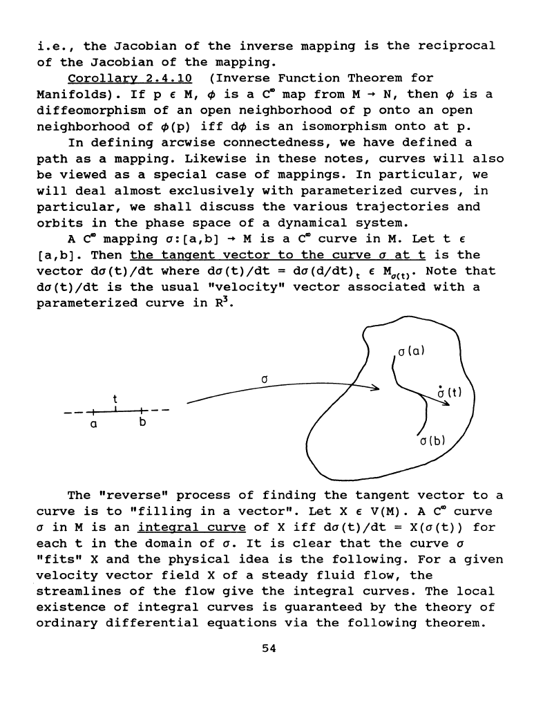
A
CU
mapping
a:
[a,b]
~
M
is
a
CU
curve
in
M.
Let
t E
[a,b].
Then
the
tangent
vector
to
the
curve
a
at
tis
the
vector
da
(t)
/dt
where
da
(t)
/dt
=
da
(d/dt)
t E
Ma<t>.
Note
that
da(t)/dt
is
the
usual
"velocity"
vector
associated
with
a
parameterized
curve
in
R
3
•
t
~tl
a(bl
a
b
The
"reverse"
process
of
finding
the
tangent
vector
to
a
curve
is
to
"filling
in
a
vector".
Let
X E V(M). A
CU
curve
a
in
M
is
an
integral
curve
of
X
iff
da(t)/dt
=
X(a(t))
for
each
t
in
the
domain
of
a.
It
is
clear
that
the
curve
a
"fits"
X
and
the
physical
idea
is
the
following.
For
a
given
velocity
vector
field
X
of
a
steady
fluid
flow,
the
streamlines
of
the
flow
give
the
integral
curves.
The
local
existence
of
integral
curves
is
guaranteed
by
the
theory
of
ordinary
differential
equations
via
the
following
theorem.
54
Theorem
2.4.11
Let
X f V(M)
and
let
p
be
a
point
in
the
domain
of
X.
Then
for
any
real
number
a
there
exists
a
real
number
r > 0
and
a
unique
curve
a:(a-r,
a+r)
~
M
such
that
a(a)
=
p,
and
a
is
an
integral
curve
of
X.
As
we
shall
see,
dynamical
systems
are
often
governed
by
the
type
of
equations
for
integral
curves,
i.e.,
da(t)jdt
=
X(a(T)).
An
integral
curve
is
called
a
trajectory
or
orbit
of
the
system.
We
shall
come
to
these
again
later.
It
is
also
convenient
to
define
a
broken
CD
curve
a
on
an
interval
[a,b)
to
be
a
continuous
map
a
from
[a,b)
into
M
which
is
~
on
each
of
a
finite
number
of
subintervals
[a,
b
1
) , [ b
1
, b
2
) ,
••
, [
bk_
1
,
b]
.
Let
X f
V(M),
we
associate
with
X a
local
one-parameter
group
of
transformations
T,
which
for
every
p f M
and
t € R
sufficiently
close
to¢
assigns
the
points
T(p,t)=
a(t)
where
a
is
the
integral
curve
of
X
starting
at
p.
Theorem
2.4.11
tells
us
that
for
every
p
there
is
a
positive
number
r
and
a
neighborhood
U
of
p
such
that
T
is
defined
and
CD
on
Ux(-r,r).
From
our
notation,
since
the
real
numbers
used
as
the
second
variable
of
T,
are
parameter
value
along
a
curve,
they
must
satisfy
additive
property,
that
is:
if
q E U,
t,
s,
s+t
€
(-r,r)
then
T(T(q,t),s)
=
T(q,s+t).
The
set
of
pairs
(p,t),
p f
M,
t f
I,
is
an
open
subset
of
MxR
containing
p,
hence
a
smooth
manifold
~x
of
dimension
m+1.
The
mapping
a:
~x
~
M
by
(p,t)
~
a(t)
is
the
flow
of
X.
Since
M
and
X
are
~,
so
the
flow
is
also
CD.
Let
us
look
at
this
description
in
terms
of
fluid
flow
again.
As
before,
let
us
suppose
that
the
fluid
is
steady
state,
i.e.,
the
velocity
of
the
fluid
at
each
point
p € M
is
independent
of
time
and
equal
to
the
value
X(p)
of
the
vector
field.
In
this
case,
the
integral
curves
of
X(p)
are
the
paths
followed
by
the
particles
of
the
fluid.
Now
let
¢(p,t)
be
the
point
of
M
reached
at
time
t
by
a
particle
of
the
fluid
which
leaves
pat
time
o.
We
notice
that
¢(p,O)
is
always
p.
Since
velocity
is
independent
of
time,
¢(q,s)
is
the
point
reached
at
time
s+t
by
particle
starting
at
q
at
timet.
If
we
put
q =
¢(p,t),
so
the
particle
started
from
55
the
point
p
at
time
o,
we
can
conclude
that
~(~(p,t),s)
=
~(p,s+t).
Also,
the
smoothness
of~.
as
functions
of
p
and
t,
will
be
influenced
by
the
smoothness
of
X.
A
p-dimensional
distribution
on
a
manifold
M
(p
S
dim
M)
is
a
function
D
defined
on
M
which
assigns
to
each
m e M a
p-
dimensional
linear
subspace
D(m)
of
~·
A
p-dimensional
distribution
D
on
M
is
of
class
c-
at
m e M
if
there
are
c-
vector
fields
X
1
,
•••
,
XP
defined
in
a
neighborhood
U
of
m
and
such
that
for
every
n e U, X
1
(n),
•••
, XP(n)
span
D(n).
An
integral
manifold
N
of
D
is
a
submanifold
of
M
such
that
di(N")
=
D(i(n))
for
every
n
eN.
We
say
that
a
vector
field
X
belongs
to
the
distribution
D
and
write
X e
D,
if
for
every
min
the
domain
of
X,
X(m)
e D(m). A
distribution
Dis
involutive
if
for
all
c-
vector
fields
X,
Y
which
belong
to
D,
we
have
[X,Y] e
D.
A
distribution
D
is
integrable
if
for
every
m e M
there
is
an
integral
manifold
of
D
contaning
m.
It
is
easy
to
see
that
an
integrable
c-
distribution
is
involutive.
Clearly,
every
one-
dimensional
c-
distribution
is
both
involutive
and
integrable,
by
the
existence
of
integral
curves.
We
would
like
to
mention
the
classical
theorem
of
Frobenius:
Theorem
2.4.11
A
c-
involutive
distribution
Don
M
is
integrable.
Furthermore,
through
every
m e M
there
passes
a
unique
maximal
connected
integral
manifold
of
D
and
every
other
connected
integral
manifold
containing
m
is
an
open
submanifold
of
this
maximal
one.
The
following
local
theorem
gives
more
information
as
to
how
the
integral
manifolds
are
situated
with
respect
to
each
other:
Theorem
2.4.12
If
D
is
a
c-
involutive
distribution
on
M,
and
me
M,
then
there
is
a
coordinate
system
(x
1
,
•••
,
xd)
on
a
neighborhood
of
m,
such
that
X;(m) = 0
and
for
every
m'
in
the
coordinate
neighborhood
the
slice
{p
e
Ml
X;(P) =
X;(m')
for
every
i
>dim
D}
is
an
integral
manifold
of
D,
when
given
the
obvious
manifold
structure
induced
by
the
coordinate
map.
56

Before
we
take
off
from
the
concept
of
flow
to
the
basic
idea
of
dynamical
systems
and
structural
stability,
we
should
prepare
ourselves
with
more
conceptual
notions
and
tools
in
differential
geometry
so
that
when
we
are
facing
the
geometric
theory
of
differential
equations,
which
is
an
integral
part
of
dynamical
systems
as
we
have
pointed
out
earlier,
we
will
be
ready
for
it.
There
are
several
topics
we
would
like
to
briefly
discuss,
namely
critical
values,
Morse
Lemma,
groups
and
group
action
on
spaces,
fiber
bundles
and
jets,
and
differential
operators
on
manifolds.
These
last
two
subjects
will
be
discussed
in
Chapter
3.
2.5
Critical
points,
Morse
theory,
and
transversality
The
idea
of
critical
points
to
be
introduced
here
is
an
extension
of
the
concept
of
maxima
and
minima
of
a
function.
As
we
know
in
calculus,
if
a
differentiable
function
f
of
one
variable
x
has
a maximum
of
minimum
for
x = x
0
,
then
dfjdx
= o
at
x
0
•
Similarly,
if
a
function
of
two
variables
x,
y
has
a maximum
or
minimum
at
(x
0
,
y
0
),
then
af;ax
=
af;ay
= o
at
this
point.
Geometrically,
what
we
are
saying
is
that
the
tangent
plane
to
the
surface
z =
f(x,y)
is
horizontal
at
(x
0
,
y
0
).
Of
course
the
same
condition
is
also
satisfied
at
a
saddle
point,
a
point
that
behaves
like
a
maximum when
approached
in
one
way
and
like
a minimum when
approached
in
another.
Moreover,
this
situation
can
be
thought
of
as
corresponding
to
an
embedding
of
M
in
3-space
such
that
the
function
f
is
identified
with
one
of
the
coordinates
z,
and
the
horizontal
plane
z =
f(x
0
,
y
0
)
is
a
tangent
plane
toM
at
(X
0
,
y
0
,
f(x
0
,y
0
)).
More
precisely,
we
have
the
following
definitions.
Let
~.
N"
are
em-manifolds,
and
f
is
a
em
map. A
point
a E
~is
a
critical
point
off
if
df
8
= o,
(i.e.,
df
is
not
onto
at
a,
or
the
Jacobian
matrix
representing
df
has
rank
less
than
the
maximum
(n)).
beN"
is
a
critical
value,
if
b
=
f(a)
for
a E
~-
A
value
b
is
a
regular
value
if
f-
1
(b)
contains
no
critical
points.
Thus
f maps
the
set
of
critical
points
onto
the
set
of
critical
values.
57
For
example,
if
M = N = R
1
,
then
a
critical
point
is
a
point
where
the
derivative
vanishes.
In
calculus
or
advanced
calculus,
the
main
interest
in
critical
point
and
critical
value
is
centered
on
the
search
for
extrema.
Although
they
are
important
in
their
applications,
they
are
of
equal
importance
in
answering
geometric
questions
such
as
the
immersions,
submanifolds,
and
hypersurfaces
as
the
following
theorem
illustrates.
Theorem
2 •
5.
1
Let
f:
MD
-+
N"
be
a
C"
map
and
b e
N"
be
a
regular
value.
Then
f"
1
(b)
is
a
submanifold
of
MD
whose
dimension
is
(m-n).
Next
we
use
a
special
but
remarkably
simple
notion
of
Lebesgue
measure
in
real
analysis.
This
particular
notion
of
measure
zero
gives
us
a
very
simple
yet
intuitive
definition
for
our
purpose
without
resorting
to
a
host
of
machinery.
Let
Wi
be
a
cube
in
R"
and
denote
its
volume
by
~(Wi).
A
set
S
~
R"
is
said
to
have
measure
zero,
~(S)
= o,
if
for
any
given
E >
0,
there
is
a
countable
family
of
Wi
such
that
(i)
s
~
uiwi;
(ii)
:r:
1
~CWi)
<
e.
It
should
be
noted
that
it
is
possible
for
the
continuous
(C")
image
of
a
set
of
measure
zero
to
have
positive
measure
(Royden
1963].
Nonetheless,
such
a
possibility
is
excluded
when
the
maps
are
C"
as
the
following
theeorem
shows.
Theorem
2.5.2
Let
S
~
U
~
R",
where
~(S)=
0
and
U
is
open,
and
let
f:
U-+
Rm
be
cr
(r
~
1).
Then
~(f(S))=
o.
Theorem
2.5.3
(Sard)
Let
f:
M
-+
N
be
C".
Then
the
set
of
critical
values
of
f
has
measure
zero
in
N.
Let
C
be
the
set
of
critical
points
of
f,
then
f(C)
is
the
set
of
critical
values
of
f,
and
the
complement
N -
f(C)
is
the
set
of
regular
values
of
f.
Since
M
can
be
covered
by
countable
neighborhoods
each
diffeomorphic
to
an
open
subset
of
Rm,
we
have
Corollary
2.5.4
(Brown)
The
set
of
regular
values
of
a
C"
map
f:
M
-+
N
is
everywhere
dense
in
N.
Corollary
2.5.5
Let
f:
MD-+
N"
(n
~
1)
be
onto
and
C".
Then
except
for
a
subset
of
N"
of
measure
zero,
for
all
y e
58

N",
f"
1
(y)
is
a
submanifold
of
M.
Moreover,
there
is
always
some y E
N"
such
that
f"
1
(y)
is
a
proper
submanifold
of
M.
Corollary
2.
5.
6
Let
the
n-disk
be
D"
= { x E
R"
I
II
x
II
S
1}
and
its
boundary
aD"
=
S""
1
'
an
(n-1)
-sphere.
Let
i:
S""
1
....
D"
be
the
inclusion
map.
Then
there
is
DQ
continuous
map
r:
D"
-+
S""
1
such
that
r-
i =
id
on
s"-
1
,
i.e.
,
no
continuous
r
such
that
for
each
x E
s"-
1
,
r(i
(x))
=
x.
If
such
an
r
exists,
it
is
called
a
retraction
of
D"
onto
s"-
1
•
For
n =
2,
this
corollary
can
be
worded
as
follows:
The
circle
is
not
a
retraction
of
the
closed
unit
disk
(normally
a
theorem
in
elementary
homotopic
theory).
As
a
corollary:
Any
continuous
map f
of
the
closed
disk
into
itself
has
a
fixed
point,
i.e.,
f(x
0
)
= X
0
for
some X
0
ED'.
This
is
the
n = 2
case
of
the
Brouwer
Fixed
Point
Theorem.
Corollary
2.5.7
(Brouwer
Fixed
Point
Theorem)
Let
D"
=
{x
E
R"l
llxll
S 1}
be
the
n-disk,
let
f:
D"
-+
D"
be
continuous.
Then
f
has
a
fixed
point,
i.e.,
there
is
some X
0
E
D"
such
that
f
(X
0
)
= X
0
•
It
has
been
realized
for
some
time
that
a
topological
space
can
often
be
characterized
by
the
properties
of
continuous
functions
on
it.
But
it
was
Morse
(1934)
who
first
called
attention
to
the
importance
of
nondegenerate
critical
points
and
invariant
index,
which
completely
characterizes
local
behavior
near
that
point.
Moreover,
the
number
of
critical
points
of
different
indices
relates
to
the
topology
of
the
manifold
by
means
of
the
Morse
inequalities.
In
addition,
a
sufficiently
isolated
critical
point
indicates
the
addition
of
a
cell
to
the
cell
decomposition
of
the
manifold.
Consequently,
this
shows
how
a
manifold
is
put
together,
as
a
cell
complex,
in
terms
of
the
critical
points
of
a
sufficiently
well
behaved
function.
On
the
other
hand,
Morse
theory
also
treats
geodesics
on
a
Riemannian
manifold.
Although
Morse
did
a
great
deal
more,
here
we
shall
only
touch
on
a few
items
directly
concerning
our
main
emphasis.
There
is
some
material
from
algebraic
topology,
such
as
homology,
Betti
numbers,
Euler
characteristics,
which
will
be
needed
when
we
get
to
the
59
Morse
inequalities.
At
the
appropriate
places,
we
shall
state
all
the
basic
facts
without
proof.
Let
us
recall
the
concept
of
a
critical
point.
Let
M
be
a
m-dimension
~
manifold
and
f:
M
~
R
be
a
~
function.
Then
a e M
is
a
critical
point
of
f
if
f
is
not
onto
at
a.
Since
the
range
of
df
is
a
!-dimension
vector
space
at
a,
a
is
a
critical
point
when
df
is
the
zero
map
at
a.
From a
more
conventional
viewpoint,
a e M
is
a
critical
point
if
there
is
a
coordinate
chart
rf>,.
:
u,.
~
Rm,
x e
u,.
such
that
all
first
partial
derivatives
of
f·
rf>,.-
1
vanish
at
rf>,.(a). And
a
real
number
b =
f(a),
where
a
is
a
critical
point,
is
called
a
critical
value.
Clearly,
the
first
partial
derivatives
at
a
critical
point
have
degenerate
behavior.
Nonetheless,
when
the
second
partial
derivatives
are
better
behaved,
it
is
called
a
nondegenerate
critical
point.
More
precisely,
if
a e M
is
a
critical
point
for
f:
M-+
R, f e
F(M),
and
a>
(f·rp,.-
1
)/ax;axi~
the
Hessian
at
a,
is
non-singular,
then
a
is
a
nondegenerate
critical
point
of
f.
It
can
be
shown
that
this
definition
is
independent
of
the
choice
of
the
coordinate
chart.
For
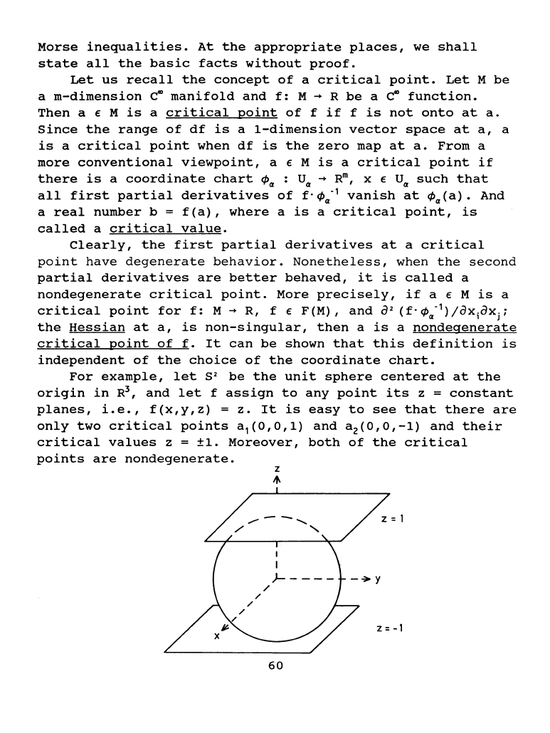
example,
let
S
2
be
the
unit
sphere
centered
at
the
origin
in
R
3
,
and
let
f
assign
to
any
point
its
z =
constant
planes,
i.e.,
f(x,y,z)
=
z.
It
is
easy
to
see
that
there
are
only
two
critical
points
a
1
(o,O,l)
and
a
2
(0,0,-1)
and
their
critical
values
z =
±1.
Moreover,
both
of
the
critical
points
are
nondegenerate.
z
.,.
60

As
another
example,
let
T
2
be
a
2-dimension
torus
imbedded
as
a
submanifold
of
R
3
•
This
T
2
can
be
thought
of
as
the
surface
traced
by
the
circle
of
center
(2,0)
and
radius
1
in
the
(x,y)-
plane
as
this
plane
is
rotated
about
the
y-axis.
The
surface
has
the
equation
(X
2
+ y• + Z
2
+
3)
2
=
16(X
2
+ Z
2
).
It
is
easy
to
show
(and
easy
to
see
from
the
figure)
that
there
are
just
four
z =
constant
horizontal
planes
H
1
,
Hz,
H
3
,
and
H
4
that
are
tangent
planes
of
T
2
at
p
1
,
Pz• p
3
and
p
4
respectively,
coresponding
to
four
critical
points
for
the
function
z
on
T
2
and
H;
(i=1,2,3,4)
are
critical
levels.
Furthermore,
one
can
show
that
these
four
critical
points
P;
(i=1,2,3,4)
are
nondegenerate.
Notice
that,
in
this
example,
if
Nc
is
a
non-critical
level
of
z,
it
is
surrounded
by
neighboring
noncritical
levels,
all
of
which
are
homeomorphic
to
each
other.
For
example,
see
the
above
figure,
between
H
1
and
Hz
all
the
noncritical
levels
are
circles.
But
as
soon
as
we
cross
a
critical
level,
a
change
takes
place.
The
noncritical
levels
immediately
below
Hz
are
quite
different
from
those
immediately
above.
In
fact,
this
observation
is
valid
in
general.
61

Let
the
differentiable
manifold
M
be
a
2-sphere
and
take
a
zero-dimension
sphere
s·
in
M.
s•
has
a
neighborhood
consisting
of
two
disjoint
disks.
This
is
of
the
form
s•xE
2
•
(E
2
is
a
2-
dim
disk).
Let
us
call
this
neighborhood
B.
Then
M
-Int
B
is
a
sphere
with
two
holes
in
it.
E
1
xs
1
is
a
cylinder
(here
E
1
is
a
line
segment),
and
when
its
ends
are
attached
to
the
circumferences
of
the
two
holes,
the
resulting
surface
is
a
sphere
with
one
handle,
i.e.,
a
torus.
Thus
the
torus
can
be
obtained
from
the
2-sphere
by
a
spherical
modification
of
type
o.
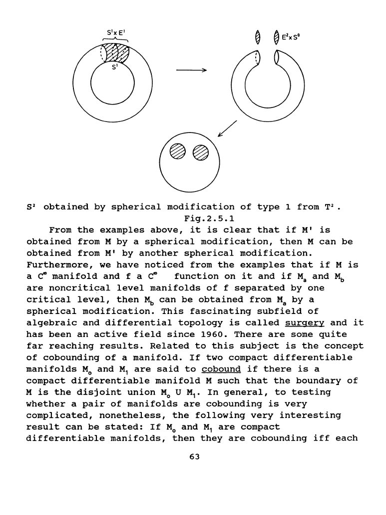
See
Fig.2.5.1.
Let
us
define
this
term
as
in
the
following:
Let
N
be
an
n-dim
~
manifold
and
sr
is
a
directly
embedded
submanifold
of
M.
sr
has
a
neighborhood
in
M
which
is
diffeomorphic
to
srxEn·r
and
we
call
it
B,
where
En·r
is
a
(n-r)
-cell.
The
boundary
of
B
is
the
manifold
srxsn·r-
1
•
Thus
M -
Int
B
is
a
manifold
with
boundary
and
the
boundary
is
srxsn·r·
1
•
But
srxsn·r-
1
is
also
a
boundary
of
the
~
manifold,
Er+
1
xsn·r·
1
•
So
the
two
manifolds
M
-Int
B
and
Er+
1
xsn·r·
1
can
be
joined
together
by
identifying
their
boundaries.
such
a
joined
space
is
a~
manifold
M'.
M'
is
said
to
be
obtained
from
M
by
a
spherical
modification
of
s
M-Int
8
T
2
obtained
by
spherical
modification
of
type
o
from
s•
•
62
s•
obtained
by
spherical
modification
of
type
1
from
T• •
Fig.2.5.1
From
the
examples
above,
it
is
clear
that
if
M'
is
obtained
from
M
by
a
spherical
modification,
then
M
can
be
obtained
from
M'
by
another
spherical
modification.
Furthermore,
we
have
noticed
from
the
examples
that
if
M
is
a
ca
manifold
and
f a
ca
function
on
it
and
if
M
8
and
Mb
are
noncritical
level
manifolds
of
f
separated
by
one
critical
level,
then
~
can
be
obtained
from
M
8
by
a
spherical
modification.
This
fascinating
subfield
of
algebraic
and
differential
topology
is
called
surgery
and
it
has
been
an
active
field
since
1960.
There
are
some
quite
far
reaching
results.
Related
to
this
subject
is
the
concept
of
cobounding
of
a
manifold.
If
two
compact
differentiable
manifolds
M
0
and
M
1
are
said
to
cobound
if
there
is
a
compact
differentiable
manifold
M
such
that
the
boundary
of
M
is
the
disjoint
union
M
0
U M
1
•
In
general,
to
testing
whether
a
pair
of
manifolds
are
cobounding
is
very
complicated,
nonetheless,
the
following
very
interesting
result
can
be
stated:
If
M
0
and
M
1
are
compact
differentiable
manifolds,
then
they
are
cobounding
iff
each
63