Kurfess T.R. Robotics and Automation Handbook

Подождите немного. Документ загружается.

-10 Robotics and Automation Handbook

from q to p is the uncertainty channel with the scalar scaled complex uncertainty δ

. The channel from w

to z

and z

is the performance channel. If we adopt q and w as the input variables, and p, z

, and z

as the

output variables, then from Figure 15.4 we may determine the interconnecting transfer function matrix H













= H





, H







−W







(15.27)

According toµ-analysis theory[19], to havetheobjectives(15.19), (15.20),and (15.26)robustlysatisifed,

it is sufﬁcient if the structured singular value of the transfer function matrix H

satisﬁes

sup



) < 1 (15.28)

for the extended plant perturbation structure





1×2

0 δ



(15.29)

where δ

denotes a complex uncertainty of dimension 1 ×2.

The objective of µ-synthesis is to construct a controller C

which stabilizes the feedback loop shown in

Figure 15.4 and yields Equation (15.28). If such a controller exists, robust stability and robust performance

are realized. The controller can be calculated using the routines provided, for example, in the µ-Analysis

and Synthesis Toolbox for Matlab [20]. Design of such a controller will be demonstrated in the case study.

15.4 Case-Study: Motion Control of the RRR Direct-Drive

Manipulator

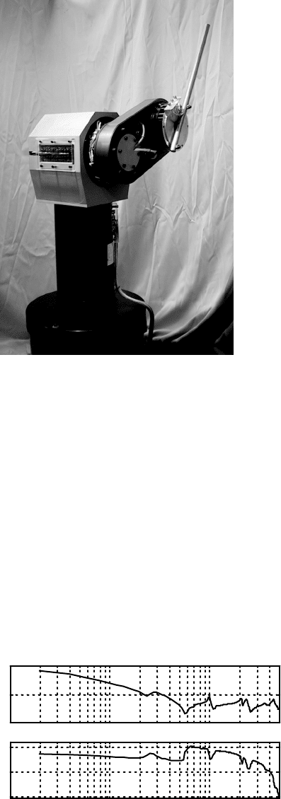
The RRR robotic manipulator (Figure 15.5) described in the chapter on modeling and identiﬁcation is the

subject of the case-study. The models of the manipulator kinematics and dynamics are available in closed-

form. The kinematic parameters were obtained by direct measurements, while the inertial and friction

parameters were estimated with sufﬁcient accuracy. Both models are used for motion control of the RRR

robot: the kinematic model computes the reference joint motions given a trajectory of the robot-tip; the

rigid-body dynamic model is used in the control laws (15.10) and (15.11) to compensate for nonlinear

dynamic couplings between the robot joints.

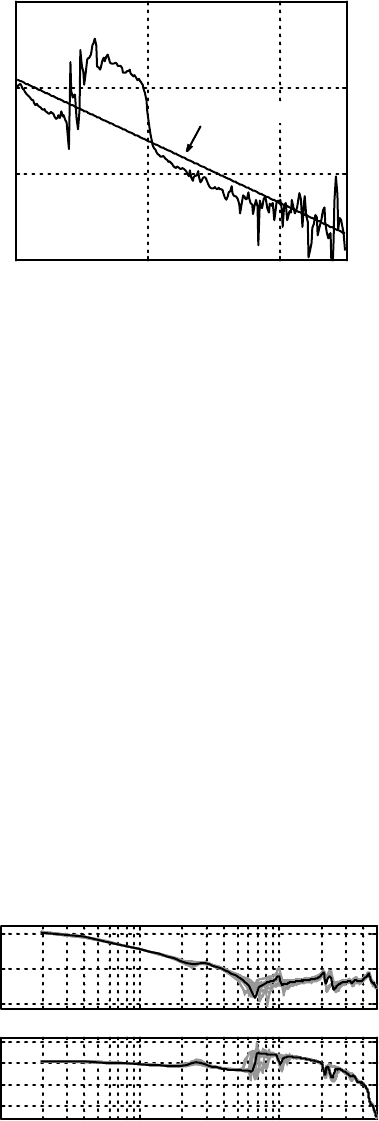
Because the dynamic model covers only rigid-body dynamics, it cannot counteract ﬂexible effects. To

illustrate this, we may inspect the FRF shown in Figure 15.6. It was determined for the ﬁrst robot joint using

the identiﬁcation procedure explained in the previous chapter. The sampling period in the identiﬁcation

experiment was T

= 1 ms. During identiﬁcation, joints 2 and 3 were kept locked such that the distal

links were fully stretched upwards. As obvious from the magnitude plot, the rigid dynamics hold only at

lower frequencies, where the −2 slope can be observed as from 28 Hz, ﬂexible effects become apparent.

A modest resonance at 28 Hz is caused by insufﬁcient stiffness in mounting the robot base to the ﬂoor. If

excited, it may cause vibrations of the robot mechanism and thus degrade robot performance. At higher

frequencies, we may observe more profound resonances. Location and damping factors of these resonances

are different for other positions of joints 2 and 3.

Apart from ﬂexibilities, an additional peculiarity of the RRR dynamics can be observed by inspection of

the phase plot shown in Figure 15.6: a frequency dependent phase lag, superimposed to the phase changes

due to ﬂexibilities. The phase lag can be related to the time-delay between the feedback control action and

the joint angular response. The time-delay can be easily identiﬁed from the FRFs measured in the third

joint, as these contain less ﬂexible effects. The phase plot shown in Figure 15.7 illustrates how the delay has

Motion Control by Linear Feedback Methods 15

-11

FIGURE 15.5 The RRR robot.

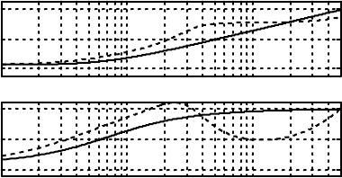
been identiﬁed. The phase is plotted linearly against the frequency to reveal a linear phase lag. The linear

lag can be described as −360

◦

δ f ,whereδ is the time-delay and f is the frequency in Hz. As the phase

drops for 360

◦

until 500 Hz, it follows that δ = 1/500 = 2 ms, i.e., δ = 2T

. The same time delay is also

present in the other two joints. Resonance effects and time-delay are problems often met in practice, and

they can be captured by the modelling part of the control design.

Feedback controllers should realize stabilization and desired performance of the manipulator motions.

Two practical designs of these controllers are demonstrated in this section. The conventional feedback

design will be presented ﬁrst, just to illustrate its limited effects on motion performance in the presence of

parasitic effects and disturbances. Then, design ofa robustfeedback via µ-synthesis willbe demonstrated. It

is sufﬁcient to present the designs for the ﬁrst robot joint only, as similar ones are applied to the other joints.

Both feedback designs use the loop-shaping methodology explained in subsection 15.3.2, which means

that the compensation of the manipulator nonlinear dynamics is performed via feedback linerization

−150

−95

−40

1 10 100

−700

−400

−100

Frequency (Hz)

Magnitude (dB)

Phase (

)

FIGURE 15.6 Flexible dynamics measured in the 1st joint.

-12 Robotics and Automation Handbook

0 200 400 500

−600

−400

−200

Frequency (Hz)

Phase (

)

Phase lag of −360

FIGURE 15.7 Phase plot of dynamics measured in the third joint reveals time delay of 2T

(15.11). Additionally, these designs assume availability of the nominal plant model. Calculation of this

model is demonstrated next.

15.4.1 Nominal Plant Model

To determine a nominal model of the dynamicsin the ﬁrstjoint,weﬁrstidentifyFRFs G

( j ω)(k =1, ..., N

)

for N

=16 static positions in the joints 2 and 3: [0 0], [0 π/2], . . . , [3π/23π/2] [rad]. These positions

span a complete revolution in both joints. The identiﬁcation is done under closed-loop conditions, as

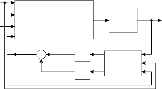
explained in the previous chapter. The identiﬁed FRFs are depicted in Figure 15.8 with the grey lines. By

inspecting their magnitude plots, we may notice that they are less steep than −2 in the frequency range

up to 4 Hz. This range is within the bandwidth of the closed-loop system established in identiﬁcation

experiments. As pointed out in the chapter on modelling and identiﬁcation, the spectral components of

an FRF that are below the closed-loop bandwidth are not reliable. However, these components can be

easily determined from the slope of the FRF components that belong to the frequency range of the rigid

dynamics. Once the distinct FRFs G

( j ω)(k =1, ..., 16) are available, the nominal response G

( j ω) can

be computed using (15.17b). The obtained G

( j ω) is shown in Figure 15.8 with the black line, and it

represents the nominal plant as a set of data points. A parametric model (transfer function) of the plant

( j ω)isﬁtted to the data using an output error model structure with a least-square criterion [14]. The

−150

−100

−50

−600

−400

−200

Frequency (Hz)

Phase (

) Magnitude (dB)

FIGURE 15.8 Identiﬁed FRFs G

, ..., G

(grey) and the nominal FRF G

(black).

Motion Control by Linear Feedback Methods 15

-13

−150

−100

−50

−600

−400

−200

Frequency (Hz)

Phase (

) Magnitude (dB)

FIGURE 15.9 Bode plots of the nominal data G

(thick) and of the parametric ﬁt P

(thin).

Bode plots of G

( j ω) and of the corresponding P

( j ω) are shown in Figure 15.9. The discrepancy between

the unreliable data below 4 Hz and the ﬁt is obvious. Above 4 Hz, the ﬁt is good up to 160 Hz. In addition to

determining P

( j ω), FRFs corresponding to the cross couplings between joint 1 and the remaining joints

were measured. At each frequency within the range of the rigid dynamics (below 20 Hz), the amplitude of

( j ω) is at least two orders of magnitude higher than the amplitude of any of the interaction terms in

(15.16). To illustrate this, in Figure 15.10 we present FRFs of the dynamics in joint 1 and of the interaction

between joints 1 and 2, identiﬁed for [q

] = [3π/2 0]. Because the cross-couplings in (15.16) are

considerably smaller than the diagonal terms, it is justiﬁed to apply single-input, single-output feedback

control designs for each manipulator joint separately.

15.4.2 Conventional Feedback Control Design

The conventional PD controller is deﬁned by (15.18). Practically, the position error e

at time t is formed

as the difference between the position measurement (from the incremental encoder) and the reference

position. The measurement is usually corrupted with quantization noise. Apart from noise, the time delay

of δ = 2T

is present in the system. If this delay is associated with the position measurements, we can

formulate the following output equation:

(t) = q

(t − δ) + η

(t)(i = 1, 2, 3) (15.30)

−50

−100

−150

Frequency (Hz)

Magnitude (dB)

FIGURE 15.10 Magnitude plots of FRFs corresponding to dynamics in joint 1 (thick) and to the cross coupling

between joints 1 and 2 (thin), identiﬁed for [q

] = [3π/2 0] [rad].

-14 Robotics and Automation Handbook

110

100

Frequency (Hz)

Phase (

) Magnitude (dB)

FIGURE 15.11 Bode plots of the conventional controllers deﬁned by Equation (15.32) (solid) and Equation (15.36)

(dotted).

where

is the position measurement, and η

is the measurement noise. These may degrade the motion

performance if the feedback law (15.18) is based on the position error

(t) =

(t) − q

r,i

(t) (15.31)

i.e.,

(t) =

r,i

(t) + u

∗

(t) (15.32a)

∗

(t) =−k

p,i

(t) − k

d,i

(t) (15.32b)

Bode plots of the PD controller designed for the ﬁrst joint are shown in Figure 15.11 with the solid

lines. These plots represent the transfer function from the error (15.31) to the control input u

(t) (15.32).

The PD gains were chosen to meet the design rules r.1–r.4 (subsection 15.3.2) as closely as possible. Fine-

tuning of the gains was manually done on the real system, to minimize inﬂuences of the quantization

noise, vibrations at the base, and ﬂexibilities at higher frequencies.

Negative inﬂuence of the time delay and the measurement noise can be optimally reduced with the use

of the LQG theory [21]. This theory suggests a Kalman observer for optimal reconstruction of the motion

coordinates used in (15.18). The Kalman observer is based on the manipulator dynamics that remain after

application of the control law (15.11), with (15.18a) taken as the feedback input:

(t) =

r,i

(t) + u

∗

(t) + v

(t)

(t) = ς

(t)

(t) = q

(t − δ) + η

(t)











(i = 1, 2, 3) (15.33)

Variable v

represents the modeling error caused by imperfect compensation of the real robot dynamics

using the nonlinear part of the control law (15.11). Here, v

is a realization of the white process noise ς

ﬁltered through a single integrator [22]. The variables

and η

have been deﬁned already by (15.30).

In the design of the observer, the position error e

(t) = q

(t) − q

r,i

(t) is regarded as a state coordinate,

together with its time derivative

and v

. We determine a discrete-time system having identical solutions

with (15.33) at t = kT

(k + 1) = E

(k) + f

∗

(k) + g

)ς

(k)

(k) = c

(k) +q

r,i

(k − 2) + η

(k)



(i = 1, 2, 3) (15.34a)

Motion Control by Linear Feedback Methods 15

-15

where

(k) = [e

(k − 2), e

(k − 1), e

(k),

(k), v

(k)]

(15.34b)







010 0 0

001 0 0

001T

000 1 T

000 0 1







, f













, g













, c

= [10000]

(15.34c)

Here, k abbreviates kT

. The delayed position reference is present in the output equation of (15.34a), as

the following holds:

(k) = q

(k − 2) + η

(k) = e

(k − 2) +q

r,i

(k − 2) + η

(k).

The Kalman observer for optimal reconstruction of the motion coordinates in the presence of the

modelling uncertainty and the measurement noise has the form:

(k + 1) = E

)

(k) + f

∗

(k)

(k) =

(k) + k

(

(k) −q

r,i

(k − 2) − c

(k)) (15.35)

where

denotes updated estimate of all states, and k

isa5×1 vector of constant Kalman gains. The

observer predicts position and velocity errors at t = kT

, from the difference between the measurement

(k) and the delayed position reference q

r,i

(k − 2). The predicted coordinates are used in PD feedback:

(t) =

r,i

(t) + u

∗

(t)

(15.36a)

∗

(k) =−k

p,i

(k) − k

d,i

(k)

(15.36b)

The block-diagram in Figure 15.12 visualizes the considered approach, featuring the following vectors:

h(q

) =Q(q

)

+ τ

, u

∗

=[u

∗

]

e =[

]

e =[

]

, and

y = [

]

The matrices of position and velocity gains are formed as K

=diag[k

p,1

, k

p,2

, k

p,3

] and K

=diag[k

d,1

d,2

, k

d,3

], respectively. These gains were determined following the rules r.1–r.4 from subsection 15.3.2,

including the on-line ﬁne-tuning to reduce inﬂuence of base vibrations and high-frequency resonances.

Bode plots of the controller for the ﬁrst joint are shown in Figure 15.11 with the dotted lines. These plots

correspond to the transfer function from

(t) − q

r,i

(t − 2T

) to the control input u

(t) in (15.36a). By

inspecting the Bode plots, we may notice that at low frequencies the PD controller (15.36) introduces

RRR

robot

Kalman

observer

M ( q

)(q

+ u*) + h(q

, q

)

–

FIGURE 15.12 PD control of the RRR robot with the Kalman observer in the feedback loop.

-16 Robotics and Automation Handbook

−50

−20

Frequency (Hz)

Magnitude (dB)

−600

−400

−200

Phase (

)

FIGURE 15.13 Open-loop gains for the ﬁrst joint achieved by three loop-shaping feedback control designs: PD

deﬁned by Equation (15.32) (solid thin), PD deﬁned by Equation (15.36) (dotted), and µ-synthesis (solid thick).

a higher gain than the PD controller (15.32). The phase characteristic of the controller (15.36) is also

advancing the phase of (15.32) at low frequencies. Higher gain implies better tracking performance, while

thephase leadimplies a possibilityfor a higher cross-over frequencyin the closed-loop.These can be veriﬁed

from the Bode plots of the open-loop gains depicted in Figure 15.13. By inspection of the magnitude plots,

it is apparent that the cross-over frequency of the controller (15.32) is lower, and its gain is smaller below

the cross-over. The higher cross-over frequency of the PD deﬁned by (15.36) indicates a potential of this

controller to realize faster robot motion. The magnitudes of the sensitivity functions of both controllers

are presented in Figure 15.15. The design rule r.3 on the maximum peaking of 6 dB is obviously realized

in both cases. At the lower frequency range, the sensitivity achieved with (15.32) is above the sensitivity

achieved with (15.36), implying a better reduction of the tracking error with the latter controller. However,

the achieved performance is still below that feasible with the feedback designed by µ-synthesis, which is

presented next.

15.4.3 µ-Synthesis Feedback Control Design

The loop-shaping control design via µ-synthesis should provide motion control of robust stability and ro-

bust performance. The grey lines in Figure 15.15 present relative differences (perturbations) in magnitudes

between G

, ..., G

, and P

. By virtue of (15.25), at each ω the maximum perturbation is represented

−30

−20

−10

Frequency (Hz)

Magnitude (dB)

FIGURE 15.14 Sensitivity functions for the ﬁrst joint achieved by three loop-shaping feedback control designs: PD

deﬁned by Equation (15.32) (solid thin), PD deﬁned by Equation (15.36) (dotted), and µ-synthesis (solid thick).

Motion Control by Linear Feedback Methods 15

-17

−40

−10

Frequency (Hz)

Magnitude (dB)

FIGURE 15.15 Magnitude plots of the weighting function W

(dotted), of relative differences between P

and

, ..., G

(grey), and envelope of all differences 

(solid).

by 

. It is shown in Figure 15.15 with the bold line. The dotted line in the same ﬁgure represents the

magnitude of the parametric weighting function W

, which was chosen in accordance with (15.24). As

already emphasized, the identiﬁed FRFs are not reliable below 4 Hz, and hence W

does not bound the un-

certainty in the lower frequency range. Figure 15.16 shows the performance weightings W

and W

, that

were chosen to adequately meet rules r.1–r.4. from subsection 15.3.2. The weighting W

should enforce

integral action in the feedback controller, together with as high as possible reduction of the position error

at low frequencies. Furthermore, it should enforce attenuation of the vibrations at 28 Hz. The weighting

should enforce the high-frequency roll-off.

Finally, a feedback controller was designed using µ-synthesis that employs iterative scaling of the 2nd

order (D-scaling [19,20]) and H

∝

optimization. Five DK iterations were necessary to determine C

which

ensures robust performance speciﬁed by W

and W

. The Bode plots of the obtained C

are shown in

Figure 15.17. The controller introduces integral action at low frequencies and deals with various resonance

frequencies over a broad frequency range. Its magnitude and phase plots have more involved shapes than

the plots of the conventional controllers depicted in Figure 15.11, indicating a potential of the µ-synthesis

controller to simultaneously handle more versatile control objectives. It is also worth noticing that the

design of the µ-synthesis controllerdoes not require an explicit treatment of the time-delay problem,which

was the case with the PD feedback. The µ-synthesis design considers the delay as an inherent property of

the controlled plant, and creates an optimal controller that tackles this problem together with other control

objectives. The block diagram shown in Figure 15.18 illustrates the control approach with the µ-synthesis

controllers C = diag[C

] in the feedback loop.

High-quality fulﬁlment of several control goals with µ-synthesis is obvious from the Bode plots of

the open-loop gain and from the magnitude plots of the sensitivity function, shown in Figure 15.13 and

Figure 15.14, respectively. The cross-over frequencies achieved with the µ-synthesis controller are higher

than with the conventional feedbacks, see Table 15.1, which means that the µ-synthesis controller can

−1

−100

−50

100

Frequency (Hz)

Magnitude (dB)

FIGURE 15.16 Magnitude plots of the performance weightings W

(dashed) and W

(dash-dotted).

-18 Robotics and Automation Handbook

100

Magnitude (dB)

−100

100

Frequency (Hz)

Phase (°)

FIGURE 15.17 Bode plots of the feedback controller C

RRR

robot

−

M ( q

)(q

+ u*) + h(q

, q

)

FIGURE 15.18 µ-synthesis feedback control of the RRR robot.

realize faster motions more accurately. Only in the last joint do the PD determined by Equation (15.36)

and the µ-synthesis controller yield identical cross-over. As seen from Figure 15.13, the µ-synthesis

controller has higher open-loop gain than the PDs below the cross-over. The higher gain is due to the

integral action. Consequently, Figure 15.14 indicates smaller sensitivity with the µ-synthesis controller

than with the conventional ones below the cross-over. The higher gain and smaller sensitivity imply that the

µ-synthesis feedback will reduce the tracking error better. Beyond the cross-over, this controller reduces

peaking around 200 Hz and 410 Hz. The µ-synthesis controllers in the other two joints also achieve higher

open-loop gains and smaller sensitivities below the cross-over, as well as attenuation of high-frequency

resonances. These will be veriﬁed by experiments, presented in the next subsection.

The plots shown in Figure 15.13 and Figure 15.14 correspond to the nominal plant model P

.We

are interested how robust C

is for application within the complete conﬁguration space of the robot.

To investigate this, in Figure 15.19 we plot the complementary sensitivity, the sensitivity, and the input

sensitivity functions of the closed-loop system with the compensator C

, calculated for P

and for all

, ..., G

. The top plots show that all the complementary sensitivities are bounded from above by the

magnitude of W

, implying that the system remains stable for all postures–the condition (15.26) is satisﬁed.

The middle and the bottom plots in Figure 15.19 show the sensitivity functions and the input sensitivity

functions, respectively. In the frequency range of reliable measurements (above 4 Hz), it is obvious that

magnitudes of all the sensitivity functions are bounded with the magnitude of 1/W

, and magnitudes of all

the input sensitivity functions are bounded with the magnitude of 1/W

. Theseimply that the performance

TABLE 15.1 The Cross-Over Frequencies (in hertz)

i PD Equation (15.32) PD Equation (15.36) µ

110 1416

210 1418

310 2020

Motion Control by Linear Feedback Methods 15

-19

−50

−20

−55

−35

−15

Magnitude (dB)

120

Frequency (Hz)

FIGURE 15.19 Magnitude plots of the nominal (bold) and of the perturbed (grey) complementary sensitivity func-

tions (top), of the nominal (bold) and of the perturbed (grey) sensitivity functions (middle), and of the nominal (bold)

and of the perturbed (grey) input sensitivity functions (bottom) are all below the prespeciﬁed bounds (dotted, dashed,

and dash-dotted lines, respectively).

speciﬁcations are robustly satisﬁed, i.e., the conditions (15.19) and (15.20) are satisﬁed for all postures.

Results similar to those presented in Figure 15.19 also hold for the other two joints of the RRR robot.

15.4.4 Experimental Evaluation

The designed controllers were tested in two different experiments. In the ﬁrst experiment, the reference

motion task was deﬁned in the conﬁguration space, as shown in Figure 15.20. It required all the joints to

be displaced for π radians in 1 s, with zero initial/terminal speed and accelerations. These demand the full

0 2 46

−2

Time (s)

Angles (rad)

0246

−6

Time (s)

Speed (rad/s) (solid)

0246

−20

Acceleration (rad/s

) (dotted)

FIGURE 15.20 Reference motion task in the ﬁrst experiment.