Kurfess T.R. Robotics and Automation Handbook
Подождите немного. Документ загружается.

10
-8 Robotics and Automation Handbook
There are many formal ways to mathematically model the motions of a robot or machine tool. Chao
and Yang [4] persuasively argued for use of homogeneous transformation matrices (HTMs) because error
budgets must account for all six possible error motions of a rigid body. HTMs include six degrees of
freedom while Denavit-Hartenberg [20] notation includes only four degrees of freedom. This article will,
therefore, describe the use of HTMs for kinematic modeling of machine tools. A general form of HTM is
100X
010Y
001Z
000 1
·
10 0 0
0cos
x
−sin
x
0
0 sin
x
cos
x
0
00 0 1
·
cos
y
0 sin
y
0
0 100
−sin
y
0cos
y
0
0 001
·
cos
z
−sin
z
00
sin
z
cos
z
00
0010
0001
(10.13)
where X, Y, and Z are displacements in the x, y, and z directions and
x
,
y
, and
z
are rotations about
the x, y, and z axes. This form of HTM allows for the large rotations required to model the commanded
motions of the robot or machine tool.
HTMs can be used to model the joints in robots and machine tools. For a rotary joint, let
z
represent
the commanded motion of the joint while δ
x
, δ
y
, δ
z
and ε
x
, ε
y
, ε
z
represent the translational and
rotational error motions of the joint, respectively. Entering these symbols into the general form of HTM
(Equation (10.13)) and employing small angle approximations to simplify yields
ε
z
+ cos
z
−sin
z
ε
y
δ
x
sin
z
ε
z
+ cos
z
−ε
x
δ
y
ε
x
sin
z
− ε
y
cos
z
ε
x
cos
z
+ ε
y
sin
z
1 δ
z
0001
(10.14)
For a linear joint, let X represent the commanded motion of the joint in the x direction while δ
x
,
δ
y
, δ
z
and ε
x
, ε
y
, ε
z
represent the translational and rotational error motions of the joint, respectively.
Entering these symbols into the general form of HTM (Equation (10.13)) and employing small angle
approximations to simplify yields
1 −ε
z
ε
y
X + δ
x
ε
z
1 −ε
x
δ
y
−ε
y
ε
x
1 δ
z
000 1
(10.15)
If the linear axis is arranged so that the bearings do not move with the rigid body they support but
are instead fixed with respect to the previous body in the kinematic chain, then the ordering of the error
motions and the commanded translations must be reversed. This kind of joint is, therefore, modeled by
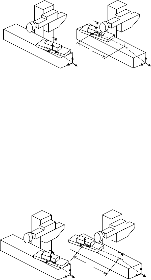
the equation below. Note the difference in Figure 10.6 and Figure 10.7. When the commanded motion X
is zero, the effect of an error motion ε
y
is the same with either Equation (10.15) or Equation (10.16). But
when X is non-zero, the error motion ε
y
causes a much larger z displacement using Equation (10.16).
Equation (10.15) is most often used in machine tool error budgets, but some linear joints are arranged
the other way, so Equation (10.16) is sometimes needed.
1 −ε
z
ε
y
X + δ
x
ε
z
1 −ε
x
δ
y
+ Xε
z
−ε
y
ε
x
1 δ
z
+ Xε
y
000 1
(10.16)
Copyright © 2005 by CRC Press LLC
Error Budgeting 10
-
9
X
The effect of angular error
motion e at the home position.
The effect of angular error
motion e with commanded motion
X
.
x
y
e
y
e
y
z
FIGURE 10.6 When the bearings are attached to the component whose motion is being driven by the joint, use
Equation (10.15) to model the commanded linear motion, X, and angular error motion, ε .
It is straightforward to modify Equation (10.14) to Equation (10.16) to model rotary and linear joints
oriented along different axes. The choice of orientation of the joints with respect to the local coordinate
systems can be made according to the context in which they are used.
To apply HTMs to construct a complete kinematic model of a robot or machine tool, one must model
the relationship of each local coordinate system in each serial chain with respect to the adjacent local
coordinate systems. Following Soons et al. [3], one may consider two kinds of HTMs in the kinematic
model, one for the joints themselves and one for the shapes of the components which are between the joints
and determine the relative location of the joints. The HTMs for the joints have already been described in
Equation (10.14), Equation (10.15), and Equation (10.16). They are labeled according to the joint number
so that the HTM for the ith joint is J
i
.
The HTMs for the shapes describe the relative position and orientation of the LCSs at the “home”
position (when the commanded motions X,
z
, etc. are zero). They are labeled according to the two LCSs
they relate to one another so that the HTM relating the ith LCS to the LCS before it in the kinematic chain
is
i−1
S
i
.
X
x
e
y
e
y
The effect of angular error
motion e at the home position.
The effect of angular error
motion e with commanded motion
X
.
y
z
x
y
z
FIGURE 10.7 Whenthe bearings are attached to the fixed component, use Equation (10.16) to model the commanded
linear motion, X, and angular error motion, ε.
Copyright © 2005 by CRC Press LLC
10
-10 Robotics and Automation Handbook
The complete kinematic model is formed by multiplying all the joint and shape HTMs in sequence.
Thus, an HTM that models a kinematic chain of n LCSs from the base to the end effector is
0
T
n
=
0
S
1
· J
1
·
1
S
2
· J
2
· ...J
n−1
n−1
S
n
(10.17)
With this HTM in Equation (10.17), one can carry out analysis of the position and orientation of any
object held by the end effector by mapping local coordinates into the base (global) coordinate system. If
the coordinates of any point on with respect to the nth LCS are (p
x
, p
y
, p
z
), then the coordinates with
respect to the base (global) LCS (p
x
, p
y
, p
z
)aregivenby
p
x
p
y
p
z
1
=
0
T
n
p
x
p
y
p
z
1
(10.18)
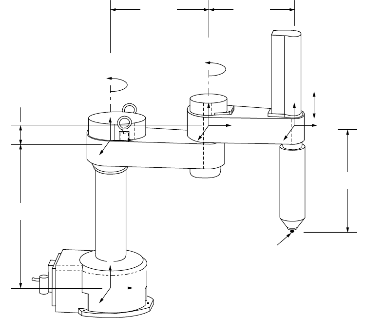
As an example of kinematic modeling, consider the SCARA type robot in Figure 10.8. Assume that the
pose depicted in the figure is the home or zero angle pose. Local coordinate systems have been assigned to
each of four major components of the robot at the location of the bearing centers of stiffness.
Joints 1 and 2 are modeled using Equation (10.14). Joint 3 is best modeled using Equation (10.16)
assuming the quill is supported by a set of bearings fixed to the arm of the robot rather than to the quill
1000 mm
500 mm 400 mm
60 mm
300 mm
Base
Point
p
Z
y
x
z
Θ
z1
Θ
z2
FIGURE 10.8 A robot to be modeled kinematically.
Copyright © 2005 by CRC Press LLC

Error Budgeting 10
-
11
TABLE 10.2 Error motions for the Example HTM Model of a SCARA Robot
Error Description µσ
ε
z1
Drive error of joint #1 0 rad 0.0001 rad
ε
z2
Drive error of joint #2 0 rad 0.0001 rad
δ
z3
Drive error of joint #3 Z · 0.0001 0.01 mm
ε
x3
Pitch of joint #3 0 rad 0.00005 rad
ε
y3
Yaw of joint #3 0 rad 0.00005 rad
xp
2
Parallelism of joint #2 in the x direction 0.0002 rad 0.0001 rad
itself. The shape transformations require translations only in this case and the translations required can
be inferred from the dimensions in Figure 10.8. Let us include only six error motions in this model as
described in Table 10.2. The resulting HTM follows the form of Equation (10.17) with alternating shape
and joint transformations
0
T
3
=
100 0mm
010 0mm
0 0 1 1000 mm
000 1
·
cos(
z1
+ ε
z1
) −sin
z1
00mm
sin
z1
cos(
z1
+ ε
z1
)00mm
0010mm
0001
·
1 0 0 500 mm
01− xp
2
0mm
0 xp
2
160mm
00 0 1
·
cos(
z2
+ ε
z2
) −sin
z2
00mm
sin
z2
cos(
z2
+ ε
z2
)00mm
0010mm
0001
·
1 0 0 400 mm
010 0mm
001 0mm
000 1
·
10ε
y3
0mm
01−ε
x3
0mm
−ε
y3
ε
x3
1 −Z − δ
z3
000 1
(10.19)
The HTM can be used to compute the location of the tip of the end effector at any location in the
working volume as a function of the joint motions and error motions.
p
x
p
y
p
z
1
=
0
T
3
0
0
−300
1
(10.20)
The resulting expressions are generally very complex. In this case the z position of the end effector is
the simplest term. It is generally safe to eliminate the second order terms — those that contain products
of two or more error motions. With this simplification, the z position of the end effector is
p
z
= 760 − Z − δ
z3
+ [400 sin
z2
]xp
2
(10.21)
Examining Equation (10.21), one can observe that the position of a point in space varies from the
commanded position according to a sum of error terms. The error terms are either linear error motions
or angular error motions multiplied by the perpendicular distance of the point of interest from the center
of rotation of each error motion.
The fact that angular error motions are amplified by perpendicular distances was formally codified
by Ernst Abb
´
e who was concerned with the effect of parallax in measurement tasks. The concept was
Copyright © 2005 by CRC Press LLC

10
-12 Robotics and Automation Handbook
later extended to machine design by Bryan [21]. As a recognition of this, large displacements caused by
small angular error motions are sometimes called “Abb
´
eerrors.” One value of the kinematic model is
that it automatically accounts for the changing perpendicular distances as the machine moves through its
working volume. In effect, the kinematic model is an automatic accounting system for Abb
´
eerrors.
Models for use in error budgeting can vary widely in complexity. The example shown in this chapter
is simple. To make the model more complete, one might also model the changing static and dynamic
loads on the machine throughout the working volume. This can be accomplished by expressing the error
motions as functions of machine stiffness, payload weight, payload position, etc.
This section has shown how to develop a formal kinematic model. The inputs to the model are the
dimensions of the machine, the commanded motions, and the error motions. The model allows one to
express the position of any point on the machine as a function of the model inputs. The next section
describes how the errors in the kinematic model combine to affect the machine’s accuracy and the overall
process capability.
10.6 Assessing Accuracy and Process Capability
A common way to characterize the accuracy of a machine is by defining one’s uncertainty about the location
of a point. The point may be the tip of an end effector, a probe, or cutting tool. The confidence can be
separately assessed at multiple points in space throughout the working volume of the machine [22]. It is
standard practice to separately characterize systematic deviations, random deviations, and hysteresis [23].
These three types of error may be described in terms of probability theory. The systematic deviations are
related to the mean of the distribution. The random deviation is related to the spread of the distribution
and, therefore, the standard deviation. The hysteresis effects can be modeled as random variation or can
be treated as systematic deviations depending on the context. A comparison of different approaches to
combining errors is provided by Shen and Duffie [24].
As an example of machine accuracy assessemnt using error combination formulae, consider the SCARA
robot modeled in the previous section. Equation (10.21) is the expression for z position of the end
effector. The commanded z position is 760 − Z. The deviation from the commanded position is −δ
z3
+
400 sin
z2
xp
2
. The deviation from the commanded position is a function of two random variables and
the commanded joint angle which is known exactly. To assess the overall effect of these two random
variables on the deviation, we may employ the combination rules for mean and standard deviation. The
mean deviation is simply the sum of the mean deviations of each term (as stated in Equation (10.6)).
−E (δ
z3
) + E ([400 sin
z2
]xp
2
) =−0.0001Z + 400 sin
z2
· 0.0002
(10.22)
The standard deviation of the z position can be estimated using the root sum of squares rule (Equa-
tion (10.7)) if we assume that the error motions are uncorrelated.
σ
2
(δ
z3
) +σ
2
([400 sin
z2
]xp
2
) =
(0.01 mm)
2
+ (400 sin
z2
· 0.0001)
2
(10.23)
We have just described a machine’s accuracy as the mean and standard deviation of a point. In many
cases, this is not a sufficient basis for evaluating accuracy. A more general definition is “the degree of
conformance of the finished part to dimensional andgeometric specifications” [25]. This definition ties
the accuracy of the machine to its fitness for use in manufacturing, making it a powerful tool for decision
making. However, to use this definition, several factors must be considered, including:
r
Sensitive directions for the task
r
Correlation among multiple criteria
r
Interactions among processing steps
r
Spatial distribution of errors
Copyright © 2005 by CRC Press LLC
Error Budgeting 10
-
13
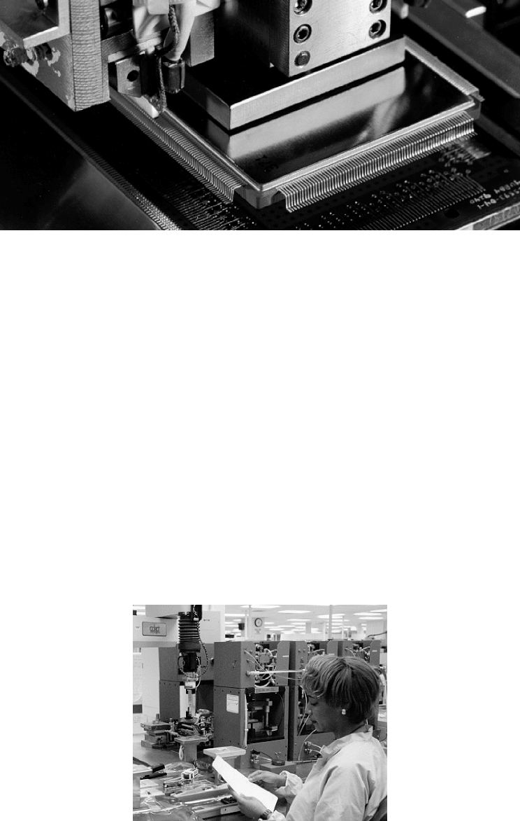
FIGURE 10.9 A robot assembles an electronic package onto a printed wiring board.
10.6.1 Sensitive Directions
The required accuracy for any particular task may be very high in one direction (a sensitive direction) as
compared with other directions. Consider a robot which must place an electronic component on a printed
wiring board (Figure 10.9). The leads extending from the package must be aligned with the pads on the
printed wiring board. This places tight requirements on the x and y position of the electronic component.
On the other hand, the flexibilityof the leads mayallow for significant errorin the z direction. Therefore, for
this assembly task, x and y are sensitive directions and z is an insensitive direction. A complete assessment
of accuracy cannot generally be made without consideration of sensitive direction for a particular task.
10.6.2 Correlation among Multiple Criteria
Thevariations due toanyindividual processingstepmayinducecorrelationamong the multiple dimensions
of the product. For example, the lead forming operation depicted in Figure 10.10 generates the “foot” shape
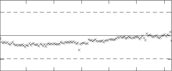
on the wire leads of an electronics package (in Figure 10.9). Errors in the lead forming process may result
in variation of the position of the leads. Figure 10.11 shows that this variation is linearly dependent on
FIGURE 10.10 An automated system for forming the leads on electronic packages.
Copyright © 2005 by CRC Press LLC
10
-14 Robotics and Automation Handbook
20
40
60
80
100
120
–1
0
1
Side #1
Lead number
Side to side error
FIGURE 10.11 Data on the location of leads formed on an automated system.
the location of the lead along the edge of the package. Correlations such as this can have a significant
impact on the process capability. Any package that has one lead out of tolerance is likely to have many
failed leads on the same side. As a result, one cannot simply multiply the probability of failure for a lead
by the number of leads to determine rolled throughput yield. Many sophisticated statistical techniques are
available to estimate yield under these circumstances, but Monte Carlo simulation is adequate for most
situations and is conceptually very simple. For each of many random trials, the error sources are sampled
from their respective distributions, the manufacturing process is simulated, and the product is compared
to the specifications. By this means, the rolled throughput yield can be estimated even if there is correlation
among multiple acceptance criteria.
10.6.3 Interactions among Processing Steps
Mostproducts undergo several processingsteps in their manufacture. Errors are transmittedthough multi-
step processes in many ways. The errors introduced by one step may be added to by subsequent processing
steps, for example, when two parts are assembled to deliver one dimension across both parts. The errors
of one step may be amplified by another step, for example, when the material properties set in one step
affect a subsequent forming operation. The errors of a previous step may be corrected to some degree by
a subsequent step, for example, the errors in the position of wire leads on an electronic component can
be compensated by robots with machine vision that place the electronic components so as to minimize
the sum squared deviation of the leads from the pads. Addition rules for error are only adequate when the
separate error terms are additive or nearly additive, so these rules should be used with care when forming
an error budget for a manufacturing system with multiple processing steps. Specialized techniques for
assessing the process capability of complex manufacturing systems, including error compensation, are
discussed by Frey et al. [6].
10.6.4 Spatial Distribution of Errors
The errors in a machine’s position at one pose may be correlated to the errors at another pose. These
patterns of correlation may be smoothly distributed across the working envelope, for example, when the
deflection due to static load rises as robot’s arm extends farther from the base. Or the patterns of correlation
may be periodic when they arise from the repeated rotations of a lead screw (see Figure 10.4). The periodic
patterns can vary in frequency, content, and phase. As described in the section on tolerancing, form and
surface finish tolerances are related to different spatial frequencies of error. One important consequence of
these facts is that the effects of individual error sources on tolerances cannot always be linearly superposed.
Copyright © 2005 by CRC Press LLC
Error Budgeting 10
-
15
HEIGHT OF THE
X AXIS CARRIAGE
1.4 µm
ROUNDNESS
ERROR
1.5 µm
ROUNDNESS
ERROR
+
=
SUPERPOSED ERRORSCUMULATIVE LEAD ERROR
1.5 µm
ROUNDNESS
ERROR
FIGURE 10.12 Superposition of two error sources and their effects on roundness.
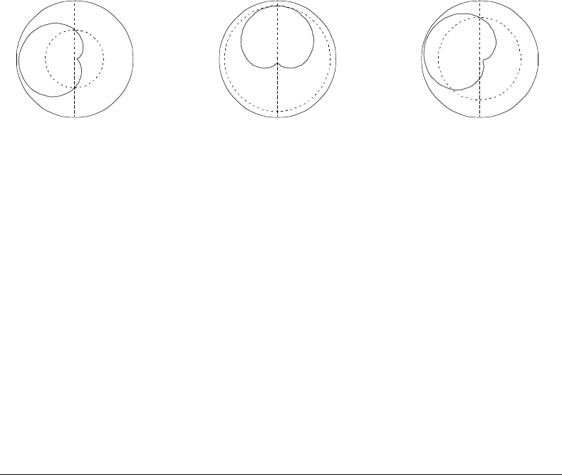
Figure 10.12 shows the effect of two error sources applied separately in an error budget for a crankpin
grinding operation. The polar plots indicate the deviation of the location of points on the surface as a
function of angular position. Figure 10.12 shows that when the two errors are superposed, the effect on
form tolerance is not additive. For tolerances of form, a root sum of squared combination rule may be
used but could prove to be overly conservative. A more precise assessment of process capability requires
direct simulation of the manufacturing process under a range of error source values.
This section demonstrated the application of error combination rules from probability theory to simple
error budgets. It also pointed out some common scenarios in which these combination rules should not
be applied. If the error in the final product is not a linear function of the error sources, a more general
probabilistic simulation may be required.
10.7 Modeling Material Removal Processes
Material removal processes are a commercially important class of manufacturing operations which present
special challenges for error budgeting. As discussed in the previous section, sensitive directions have a
profound impact on the mapping between error motions and accuracy of the finished part. In machining,
only motions normal to the surface of the part are sensitive. Error motions parallel to the surface of the
part have little effect. But the sensitive directions change in complicated ways as the tool moves and even
vary across the length of the cutting tool at a single point in time. This section presents a general solution
to incorporating the geometry of material removal into an error budget.
The mapping from cutting tool positioning error into workpiece geometry error can be formulated as a
problem in computational geometry. Machining can be modeled as the sweeping of a cutting tool through
space which removed everything in its path. The mathematics of this process is described by swept envelope
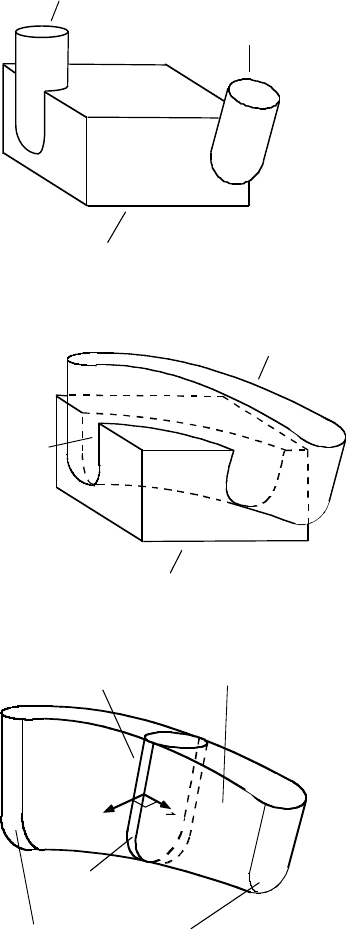
theory as illustrated by Figure 10.13. The motion of the tool is determined by the kinematic model. The
swept volume of the cutting tool is the collection of the set of points in the interior of the cutting tool as
it moved from its initial position to its final position (Figure 10.13a and Figure 10.13b). The machined
surfaces are the subset of the swept envelope of the cutting tool that lie in the interior of the workpiece
stock. The swept envelope of the cutting tool is the set of points on the surface of the swept volume. The
swept envelope consists of two types of components: a subset of the boundary of the generator at the initial
and final positions, and surfaces generated during the motion of the generator [26] (Figure 10.13c). For
many machining operations (plunge grinding, horizontal milling, etc.), only the surfaces of type 2 are of
interest. Therefore, only surfaces of type 2 will be considered here.
Wang and Wang [26] give a general method for developing an implicit formulation of the envelope
surface of a swept volume from a description of a generator curve and a motion function. The key to the
Copyright © 2005 by CRC Press LLC
10
-16 Robotics and Automation Handbook
Initial Tool Position
Final Tool Position
Workpiece Stock
(a) The cutting tool in its initial and final positions with respect to the workpiece
Swept Volume
of the Cutting Tool
Machined Workpeice
Machined Surface
(b) The swept volume of the cutting tool as it moves between the initial and final positions.
Envelope Surface
of Type 2
Critical Curve
n
^
Generator
Envelope Surfaces of Type 1
(c) The envelope surface of the cutting tool with normal and velocity vectors.
v
FIGURE 10.13 Swept envelopes of cutting tools. (a) The cutting tool in its initial and final positions with respect to
the workpiece. (b) The swept volume of the cutting tool as it moves between the initial and final positions. (c) The
envelope surface of the cutting tool with normal and velocity vectors.
method is the realization that, at any point in time, the generator curve is tangent to the envelope surface
along a “critical curve” that lies on both the generator and envelope surface. Therefore at any point (
p)
along the tangent curve, the unit normal vector to the envelope surface is identical to the unit normal
vector (
ˆ
n) of the generator at that point and at that instant in time. Further, the velocity (
v) of point
p
Copyright © 2005 by CRC Press LLC
Error Budgeting 10
-
17
must be tangent to the envelope surface. Therefore
v(p, t) ·
ˆ
n(p, t) = 0
(10.24)
Equation (10.24) above is, in effect, a procedural definition of the envelope surface of a swept solid. If one
can construct parametric formulations
v(p, t) = v(u, v, t)
(10.25)
and
ˆ
n(p, t) =
ˆ
n(u, v, t)
(10.26)
then Equation (10.24) will result in a nonlinear equation in u, v, and t which all the points on the surface
of the envelope must satisfy. Solution of Equation (10.24) is very complex in general, but with some
restrictions on the geometry of the cutting tool, a closed form solution is available which is useful for error
budgets. For example, grinding wheels and milling cutters can, under certain conditions, be modeled as
surfaces of revolution.
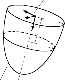
Let us assume that the z axis of the tool local coordinate system lies on the cutting tool’s axis of rotation
(Figure 10.14). The shape of the cutting tool is defined by a function r (u), equal to the perpendicular
distance of the cutting edge (or grain) from the axis of rotation as a function of u, the component along
the axis of rotation of the distance from the cutting point to the origin of the tool local coordinate system.
If the machine is modeled by two kinematic chains T (for the cutting tool) and W (for the workpiece),
then the location of the origin of the tool LCS with respect to the workpiece is
c(t) =
0
W
−1
n
·
0
T
m
· (
0001
)
T
(10.27)
The unit vector pointing along the axis of rotation of the tool is
ˆ
a(t) =
0
W
−1
n
·
0
T
m
· (
0010
)
T
(10.28)
Cutting Tool
Local Coordinate
System
Cutting Tool
(Surface of Revolution)
u
r
(
u
)
r
(0)
x
y
z
FIGURE 10.14 Representing a cutting tool as a surface of revolution.
Copyright © 2005 by CRC Press LLC
