Kristiansen Svein. Maritime Transportation: Safety Management and Risk Analysis
Подождите немного. Документ загружается.


The actual computations for the present case can partly be based on the SSD in Table 4.3
and are summarized in Table 4.4. F
calc
is computed as follows:
F
calc
¼ 680:9=ð2278:6=8Þ¼2:39
The test criteria for F
calc
are taken from a F tabulation for a specified significance
level and (
1
,
2
) degrees of freedom. Looking up the table, we have:
Assuming: ¼ 0:05
We get: F
TAB
ð0:05, 1, 8Þ¼5:32 > F
calc
¼ 2:39
It can be concluded that F
calc
is within the confidence range consistent with the H
0
hypothesis. The linear model should in other words be rejected as the b
1
coefficient is not
significantly different from zero. We should therefore stick to the simple ‘constant level’
model:
N
L&SA
¼ 202:9 ðaccidents and losses=yearÞ
4.5 CON SEQU EN CE ESTIMATION
4.5.1 Distri bution Characteristi cs
The most often used risk parameters are the accident frequency and the measure of
consequence. In this chapter we shall focus on the second parameter which has certain
important characteristics:
. The consequences of an accident may take different forms such as human injury and
loss (fatality), environmental pollution, material and economic losses.
. Accident sta tistics are mainly based on high-frequency events with minor
consequences.
. As risk managers we are more concerned with low-frequency and large-consequence
events.
. Uncritical use of accident statistics may therefore give a misleading picture of the
worst-case scenario.
Ta b l e 4 . 4 . ANO VA case
Source Sum of squares Degrees of freedom Mean square
Due to regression 680.9 1 680.9
Residual 2278.6 10 2 ¼8 284.8
Total corrected for mean 2959.6 10 1 ¼9
106 CHAPTER 4 STATISTICAL RIS K MO N IT O RI N G
Case
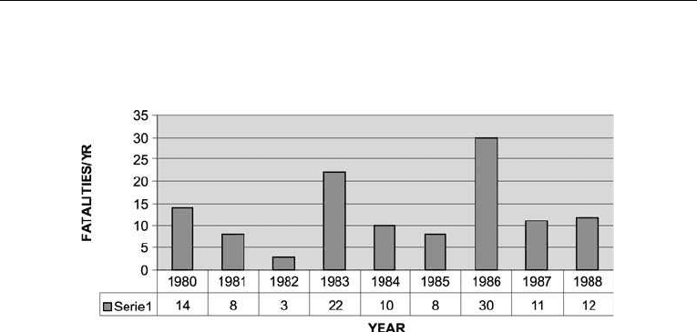
The fatality rate in the Norwegian offshore sector in the 1980s was as follows:
The following can be stated about the annual number of fatalities for this period:
Average number: 13: 1 fatalities=year
Minimum number: 3 fatalities=year
Maximum number : 30 fatalities=year
However, the tragic fact was that in 1989 we had 119 fatalities in one single accident.
One may then ask whet her the statistic figures from the previous period co uld say anything
about the probability of a catastrophe of this magnitude. The immediate answer might
be to say ‘no’, as the mean fatality number was 13.1. Even the largest fatality number
in the period was 30, which was less than 1/3 of the accident in 1989. However, if we
could establish the distributional characteristics of the fatality, the chances might
be brighter.
4.5.2 Fitting a Non-parametric Distribution
Rather than estimating the parameters of a known distribution, one may generate an
empirical distribution directly on the basis of the observed da ta. Let us take data for
the economic loss as a result of ship accidents as a case to demonstrate the approach
(Table 4.5).
A non-parametric or empirical distribution is established as follows:
1. Select ranges for the loss variable (column 1).
2. Estimate average point value for each range (column 2).
3. List the number of observations in each range N
i
(column 3). The sum of observations
is given below (N).
4.5 CONSEQUENCE ESTIMATION 107

4. Comp ute the accumulated number as follows:
AN
iþ1
¼ AN
i
þ N
iþ1
5. Comp ute the ‘artificial’ CDF value in following manner:
FðxÞ¼AN
iþ1
P
Nþ1
The ‘trick’ of adding 1 to N reflects the fact that CDF approaches the value 1.0
asymptotically.
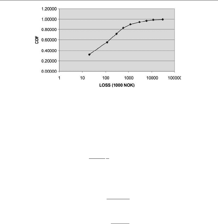
The result is shown in the right -most column. The distribution is plotted in Figure 4.10
with a logarithmic scale for the abscissa. It can be concluded by observation that the curve
fits the data reasonably well.
4.5.3 The Log-Normal Distribution
Certain consequence parameters, such as the number of lives lost or the size of an oil spill,
seem to follow a very skewed distributions. Stated simply it means that:
. Accidents with minor or lesser consequences represent the majority of the total number
of events.
. However, a limited number of accidents lead to great or catastrophic consequences.
Ta b l e 4 . 5 . Economic loss in accidents
12345
Range of X
(loss in 1000 NOK)
Point value: X Observations
N
Accumulated
N
CDF
1–100 20 48 48 0.32432
100–200 120 35 83 0.56081
200–500 300 24 107 0.72297
500–1000 600 16 123 0.83108
1000–2000 1200 10 133 0.89865
2000–5000 3000 7 140 0.94595
5000–10,000 6000 4 144 0.97297
10,000–20,000 12000 2 146 0.98649
20,000–50,000 30000 1 147 0.99324
Sum 147
Sum þ1 148
108 CHAPTER 4 STATISTICAL RIS K MO N IT O RI N G
The log-normal (LN) distribution has properties that makes it suitable for describing
consequence phenomena. If the random variable ln X is normally distributed , N (
1
,
1
),
then the variable X is said to be log-normally distributed, LN(, ). The PDF can be
expressed as follows:
fðxÞ¼
1
ffiffiffiffiffiffiffiffiffiffi
2
1
p
1
x
e
ðln x
1
Þ
2
=2
2
1
ðÞ
where
1
¼ ln
2
ffiffiffiffiffiffiffiffiffiffiffiffiffiffiffiffi
2
þ
2
p
"#
1
¼
ffiffiffiffiffiffiffiffiffiffiffiffiffiffiffiffiffiffiffiffiffiffiffiffiffi
ln
2
þ
2
2
s
The expected value and variance are given by:
EðXÞ¼e
1
þ
1
=2ðÞ
Var X ¼ e
2
1
þ
1
ðe
2
1
1Þ
Exam p le
It has been pointed out that the log-normal distribution gives a good representation of
variables that extend from zero to þ infinity. Another observation is that it models well
Figure 4.10. Economic loss per accident.
4.5 CONSEQUENCE ESTIMATION 109
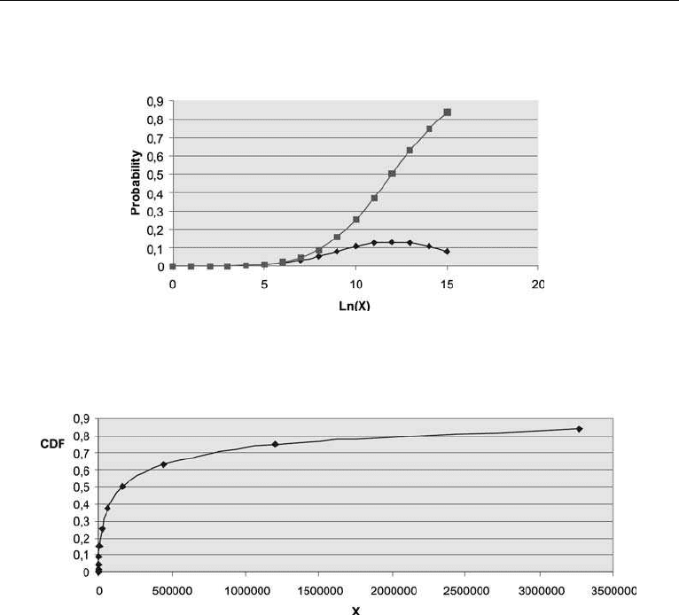
variables that are a product of other stochastic variables. The figure below shows the PDF
and the CDF for the normally distributed variable ln X, given by N(10, 2).
The corresponding CDF for X, which is log-normally distributed, is shown in the diagram
below. It is evident that distribution models a variable that may take large values.
4.5.4 Fit ting a Parametric Distri bution to O bserved Data
Vose (2000) has given some basic rules for deciding whether to apply a theoretical
distribution when we are going to model a stochastic variable. Some key points are:
. Does the theoretical range of the variable match that of the fitted distribution?
. Does the dist ribution reflect the characteristics of the observed variable?
In order to illustrate the practical approach, we will use a set of data for cargo oil outflow
as a result of ship accident (see Table 4.6).
It has been propo sed that oil outflow volume may be described by a log-normal
distribution because:
. The distribution range is positive numbers.
. It is highly skewed.
110 CHAPTER 4 STATISTICAL RISK MON ITO RING

. The outflow may be seen as a product of a number of failures: accident, load condition
and penetration of hull barrier.
In the following paragraph we will give a stepwise description of the approach applied.
The numerical computations were done with Excel and are summarized in Table 4.7.
The approach is as follows:
1. List the ranges for observed outflow amount in tonnes.
2. Select subjectively a point value X within each range.
3. List the number of observations N for each range.
4. The observed PDF value is computed as follows:
The total number of observations: N ¼22
PDF value: f(x) ¼N/(N þ1)
Table 4.6. Oil outflow dist ribution based on 22 ship accidents
Outflow size (tons) No. of observations
10–100 9
100–500 8
500–1000 2
1000–5000 1
5000–10,000 1
10,000–50,000 1
Ta b l e 4 . 7. Excel datasheet: Estimation of log-normal distribution
Range: XX Observations Observed
PDF
Observed
CDF
Estimated
CDF
Estimated
PDF
Squared
diff PDF
10–100 20 9 0.3913 0.3913 0.41628 0.41628 0.0006
100–500 200 8 0.3478 0.7391 0.69874 0.28246 0.0016
500–1000 600 2 0.0870 0.8261 0.80789 0.10915 0.0003
1000–5000 2000 1 0.0435 0.8696 0.89490 0.08701 0.0006
5000–10,000 6000 1 0.0435 0.9130 0.94546 0.05056 0.0011
10,000–50,000 20000 1 0.0435 0.9565 0.97644 0.03098 0.0004
0.0047
Mean 4803.3 Sum 22
St. dev. 7771.3 Sumþ123
1
3.66
1
3.14
4.5 CONSEQUENCE ESTIMATION 111
5. The observed cumulative value:
F
i
ðxÞ¼f
i
ðxÞþf
i1
ðxÞ, where f
0
ðxÞ¼0
The theoretical distribution function is estimated by means of the Solver function in
the Excel spreadsheet:
. Recall that the variable X is LN(, ) distributed if ln(X )isN(
1
,
1
) distributed.
. The first step is to select a set of arbitrary values for
1
and
1
.
. These values are entered into the function that is found under the Excel function
menu. The function returns the CDF value F(x).
6. The estimated PDF values are simply computed by applying the following formula:
f
i
ðxÞ¼F
i
ðxÞF
i1
ðxÞ
7. The theoretical distribution is obtained by first computing the sum of squared
deviations between observed and estimated CDF values. These are shown in the
right-most column.
8. The final step is to apply the Solver function, which is a search algorithm:
. Minimize: sum of squares of deviations of PDF
. By selecting optimum values for
1
and
1
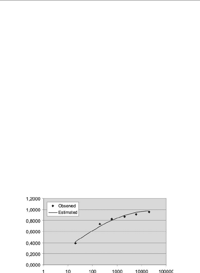
9. The solution found by Solver was:
1
¼ 3:66 and
1
¼ 3:14
The theoretical distribution function is plotted in Figure 4.11.
Figure 4.11. Oil outflow from ship accidents g iven by a log-normal distribution.
112 CH APTER 4 STATISTICAL RISK MO N IT O RI N G

4.5.5 Estimating a W orst-Case Scenario
As pointed out earlier, the risk manager is not primarily concerned about the ‘average’
accident but rather the worst-case scenario. With the previous case in mind, the problem
may be stated as follows: What is the risk of having a ship accident leading to an oil
outflow of at least 100,000 tons?
Let us assume that the frequency of accidents leading to oil spill has been studied for
a certain operation and estimated to be:
A
¼ 6 accidents=year
The probability of having a spill greater than 100,000 tons is:
PðS 100,000Þ¼1 FðS < 100,000Þ
Using the CDF in Figure 4.11 we get F(S < 100,000) ¼0.9937, or
1FðS < 100,000Þ¼0:00626
The return period is defined as the average time between events of a certain magnitude,
and may be written:
T
R
¼
1
A
PðS 100,000Þ
¼
1
A
1 FðS < 100,000Þ
½
which gives the following estimate:
T
R
¼ 1=ð6 0:00626Þ¼26:6 years
It may, however, be questioned whether this estimate is sufficiently precise.
Another way of stating the risk of this catastrophic scenario is to ask what is the
probability of having this event in any given year? This may be answered in the
following way:
1. Taking a conservative view: What is the maximum number of accidents in one year?
Assuming a Poisson distribution and a CDF value F(N
A
) ¼0.95, we obtain, by looking
up a table:
N
A
¼ 10 ðExact value: Fð10Þ¼1 0:0413 ¼ 0:9587Þ
4.5 CONSEQUENCE ESTIMATION 113

2. The next question is: What is the probability that one out of these 10 accidents will
lead to a spill greater than 100,000 tons? This can be seen as a binomial situation:
pðxÞ¼
n!
x!ðn xÞ!
p
x
ð1 pÞ
nx
pð1Þ¼
10!
1! 9!
0:00626
1
ð1 0:00626Þ
9
¼ 0:059
The risk of the catastrophic scenario on an annual basis is 6%. In other words this
is a situation that is fairly probable or at least far from being improbable! This
conclusion may therefore lead to an improvement in the operation.
3. The last point was not quite correct as there is a remote probability that even more
than one accident may lead to a spill of at least 100,000 tons. The probability that all
10 accidents give a catastrophic spill can be written:
pð10Þ¼1
10!
0! 10!
0:0026
0
ð1 0:0026Þ
10
¼ 1 0:9387 ¼ 0:061
The result is almost identical for the simple reason that having more than one
catastrophic spill is a very remote outcome.
Given the probability of 0.06 for this disaster scenario, we may estimate the
return period:
T
R
¼ 1=ð0:06Þ¼16:7 years
It can be concluded that this estimate gives a much lower return period than the first one
(26 years).
4.5.6 Extreme V alue Estimation
In many situations the risk manager is, as already pointed out, more concerned with the
worst-case situation rather than the average loss number. It may then be more feasible to
focus on the extreme values in each observation period rather than using the whole set
of data.
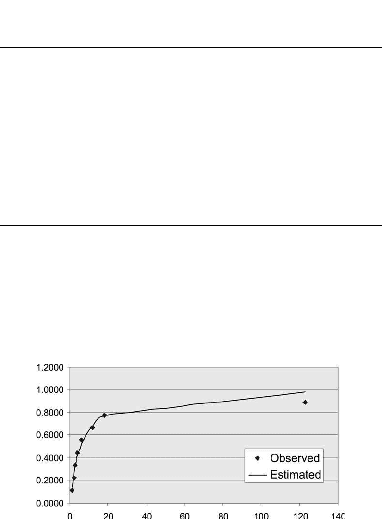
Table 4.8 reports the most serious single accident measured by the number of fatalities
for the offshore sector in the years 1973–80. It can be observed that the variation is quite
large and is best illu strated by the last two years where the number went from 1 fatality to
123 fatalities as a result of the Alexander L. Kielland loss.
It is possible to estimate a so-called extreme value distribution on the ba sis of such a
sample set. The approach is basically the same as described in the preceding section with a
few modifications.
114 CH APTER 4 STATISTICAL RISK MO N IT O RI N G
Ta b l e 4 . 8 . Maximum number of fatalities per accident: the Norwegian offshore sector,1973^ 80
Accident Year Fatalities: X
Helicopter emergency landing 1973 4
Diving bell 1974 2
Alpha capsule 1975 3
Deep Sea Driller 1976 6
Helicopter crash 1977 12
Helicopter crash 1978 18
Unspecified 1979 1
Alexander L. Kielland capsize 1980 123
Ta b l e 4 . 9. Excel sheet: estimating extreme value distribution
Observed Observed Estimated Estimated Sum of squared
Fatalities: X Rank: N CDF PDF PDF CDF deviations
1 1 0.1111 0.1111 0.1341 0.1341 0.0005
2 2 0.2222 0.1111 0.1194 0.2535 0.0010
3 3 0.3333 0.1111 0.0896 0.3430 0.0001
4 4 0.4444 0.1111 0.0699 0.4129 0.0010
6 5 0.5556 0.1111 0.1028 0.5157 0.0016
12 6 0.6667 0.1111 0.1697 0.6855 0.0004
18 7 0.7778 0.1111 0.0857 0.7711 0.0000
123 8 0.8889 0.1111 0.2046 0.9757 0.0075
N þ1 9 Sum: 0.0121
Figure 4.12. Maximum number of fatalities per offshore accident.
4.5 CONSEQUENCE ESTIMATION 115
